The purpose of this dissertation is to measure the impact of broadband speed on economic growth in 20 OECD countries. Macroeconomic indicators for this study were collected from World Bank and ITU databases, except for speed data collected by Akamai, a company that provides broadband testing and online network diagnostic application data. It is further shown that over the considered time period, returns are positive but decreasing due to rising GDP rates.
The upper threshold of speed related gains moves higher due to the "readiness". I am also grateful to the Department of Economics and all its members' staff for all the thoughtful guidance. To conclude, I cannot forget to thank my family and friends for all the unconditional support.
Introduction
- Next-generation broadband networks
- Benefit of greater broadband speed
- The concept of Broadband Speed
- Defining speed
- Measuring speed
Although the importance of broadband speed has been recognized almost everywhere, there are only a few studies that investigate this issue in the academic field, especially in empirical research. A paper investigating the impact of broadband speed on economic growth is as follows: Faster is better. The higher the video quality, the higher the broadband speed needed, not only for entertainment purposes, but it is also increasingly believed that video communication will offer some benefits in the future.
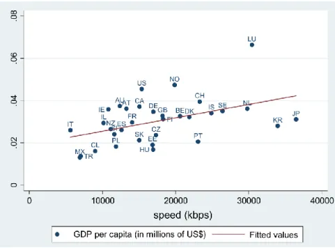
10 With these benefits from new applications and content, higher broadband speed has been emphasized through numerous reports from both the public and private sectors as contributing more benefits than lower speed broadband. To illustrate the benefits of broadband speed and economic output, the relationship between one of the economic outputs (GDP per capita) and the average broadband speed in OECD countries is presented in Figure 1. Source: Impact of broadband speed on economic output: An empirical study by the OECD - the countries of Kongaut, Chatchai;.
Therefore, the achieved broadband speed is not equal to the bandwidth, as many parameters play a role here. As seen in Figure 5, three different and respected organizations have estimated different results in terms of the three best achieved levels of broadband speed (Mbps).
Literature Review on the economic impacts of broadband internet
Contribution to economic growth
- Mass Threshold and Saturation effect
- Broadband studies and the endogeneity problem
Research aimed at generating hard evidence on the economic impact of broadband is relatively recent. The research on the impact of broadband on economic growth covers many aspects, ranging from its overall impact on GDP growth to the different impact of broadband by industrial sector, the increase in exports and changes in intermediate demand and import substitution. In addition to measuring the overall economic impact at the macro level, research on the economic impact of broadband has focused on the specific processes underlying this effect.
Does the economic impact of broadband increase with penetration and can we define a saturation threshold when there are diminishing returns to penetration. A critical element of the developing theoretical framework of broadband network externalities is the impact that levels of infrastructure penetration can have on output. The findings of the "critical mass" research on the impact of telecommunications on the economy show that the impact of broadband on economic growth can become significant only after the adoption of the platform reaches high levels of penetration.
At low broadband penetration rates, we believe that the impact of broadband on the economy is minimal due to the concept of "critical mass". For example (Koutroumpis 2009)6 found that for OECD countries the contribution of broadband to OECD economic growth increased with penetration. They find that the effect of broadband on the economy diminishes beyond a certain level of adoption (which has yet to be determined).
This effect studied for ICT also occurs with broadband. The accumulation of intangible capital and the adoption of e-business processes delay the full economic impact of broadband. More importantly, this simultaneous approach has since been applied to the case of broadband penetration in Koutroumpis (2009)5 and the spread of mobile telecommunications in Gruber and Koutroumpis (2011)12.
In addition to the simultaneous approach in previous sections, there are several studies that aim to map the impact of broadband on economic growth over the past decade using different methods. The authors transformed economic output into a growth variable, using control variables to separate the effects of broadband. Rohman and Bohlin (2012)4 were among the first to estimate the impact of broadband speed on economic output, applying Lehr et al.'s model.

Conclusions on literature review
25 dynamic regressions that include variables for GDP, the number of broadband users, the degree of urbanization and the real inflow of foreign direct investment, the authors use panel cointegration and Granger causality tests to verify causal relationships. Initially, cointegration is found between all four variables, suggesting long-term causal relationships between these variables. In contrast, the Granger causality tests do not provide evidence of any long-run causality between GDP and broadband penetration.
In the short term, the authors find that a two-way causality between economic growth and broadband penetration exists only for developed countries. To estimate the return parameters for broadband infrastructure, the authors set up a simultaneous equation model, similar to Röller and Waverman (2001)12, and use fixed-effect three-stage least squares regression. The estimates suggest that broadband adoption had a significant positive effect on GDP during the observed period.
Moreover, the results indicate that this effect is significantly greater for a broadband adoption rate of over 15 percent.
The model
Aggregate production function
While the coefficients for labor (L) and capital (K) should be typical of production functions, the coefficient of broadband penetration in equation (1) estimates the unidirectional causality flowing from the stock of broadband telecommunications infrastructure to total GDP. In order to distinguish the possible effects of broadband telecommunications infrastructure on GDP from the effects of GDP on broadband telecommunications infrastructure, I specify a micro-model for the telecommunications sector in each country consisting of an equation for the demand for broadband infrastructure.
Demand for broadband infrastructure
Data
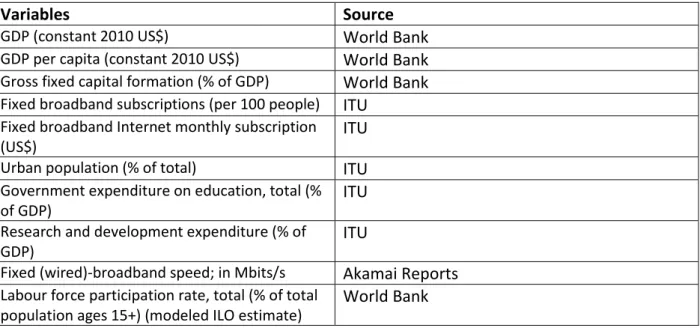
Fixed (wired) broadband speed; in Mbit/s Akamai Reports Labor participation rate, total (% of total population aged 15 years and over) (modeled ILO estimate).
Panel Data Analysis Results
- The fixed effects model
- The random effects model
- Dynamic panel data estimators
- Results
- Demand equation regression
- Aggregate production function regression (Average speed)
- Aggregate production function regression (Peak speed)
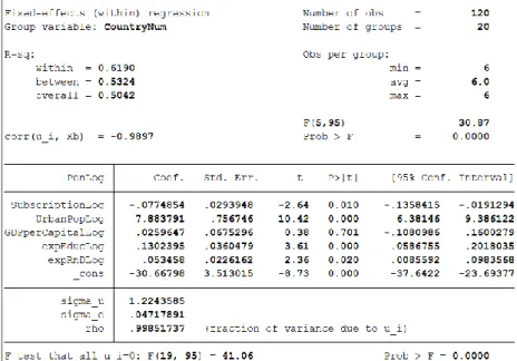
This term consists of a constant intercept, α, and individual specific errors, μi. The distinguishing feature of the fixed effects model is that δi has a real but unobserved effect that we need to estimate. This is the reason for assuming a correlation between the subject error term and the predictor variables.
The error covariance at time t and time S depends on the variance of μI and VIT. The distinguishing feature of the random effects model is that μi does not have a true value, but rather follows a random distribution with parameters that we need to estimate. It is based on the notion that the instrumental variables approach mentioned above does not exploit all the information available in the sample.
By doing this in a Generalized Method of Moments (GMM) context, we can construct more efficient estimators of the dynamic panel data model. 37 In the case of random effects panel data analysis, the interpretation of the coefficients is complicated as they include both within-unit and between-unit effects. It is used to test the hypothesis that at least one of the regression coefficients of the predictors is not equal to zero.
The number in parentheses indicates the degrees of freedom of the chi-square distribution used to test the Wald chi-square statistic and is defined by the number of predictors in the model. In other words, this is the probability of getting this chi-square statistic (89.85), or another extreme, if there is really no effect of the predictor variables. The parameter of the chi-square distribution used to test the null hypothesis is defined by the degrees of freedom in the previous row, chi2.
P>|z| – This is the probability that the z-test statistic (or a more extreme test statistic) would be observed under the null hypothesis that the regression coefficient of a given predictor is zero, given that the rest of the predictors are present in the model. In the Arellano-Bond framework, the value of the dependent variable in the previous period is a predictor of the current value of the dependent variable. Arellano-Bond suggests the second lag of the dependent variable and all possible lags after that.
The other instruments are given by the first difference of the regressors and the constant. 41 test, <0.0001, would lead us to conclude that at least one of the regression coefficients in the model is not equal to zero.
Conclusion