CRC Press is an imprint of Taylor & Francis Group, an informa Copyright © 2015 by Steven H. Visit the Taylor & Francis website at http://www.taylorandfrancis.com and the CRC Press website at http:// www. crcpress.com.
PREFACE TO THE FIRST EDITION
A broad introduction to nonlinear dynamics, for students with no prior knowledge of the subject. Here one goes straight through the entire book, covering the core material at the beginning of each chapter, selecting a few applications to discuss in depth, and giving light treatment to the more advanced theoretical topics, or skipping them altogether.
OVERVIEW
- Chaos, Fractals, and Dynamics
- Capsule History of Dynamics
- The Importance of Being Nonlinear
- A Dynamical View of the World
The invention of the high-speed computer in the 1950s was a turning point in the history of dynamics. An axis tells us the number of variables needed to characterize the state of the system.
Part I
ONE-DIMENSIONAL FLOWS
FLOWS ON THE LINE
Introduction
A Geometric Way of Thinking
You can see that there are two kinds of fixed points in Figure 2.1.1: solid black dots represent stable fixed points (often called attractors or sinks because the flow is towards them), and open circles represent unstable fixed points (also known as repellers or sources) . Armed with this picture, we can now easily understand the solutions to the differential equation xsin.
Fixed Points and Stability
This imaginary fluid is called the phase fluid, and the real line is the phase space. The appearance of the phase portrait is controlled by the fixed points x*, defined by f ( x*) 0; they correspond to the stagnation points of the flow.
Population Growth
A mathematically convenient way to incorporate these ideas is to assume that the growth rate per capita. If the population initially exceeds the carrying capacity ( N0 > K ), then N ( t ) decreases to N K and is concave up.

Linear Stability Analysis
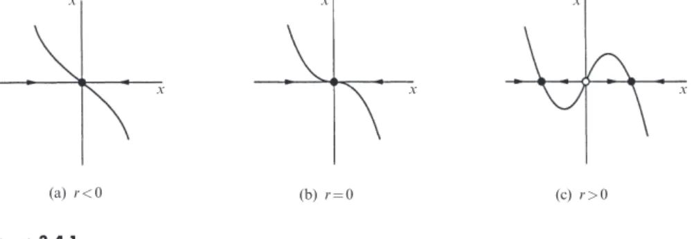
If you look back at the previous examples, you will see that the slope was always negative at a stable fixed point. Case (c) is a hybrid case, we will call semi-stable, since the fixed point attracts from the left and repels from the right.
Existence and Uniqueness
Threatened by this example, we state a theorem that provides sufficient conditions for the existence and uniqueness of solutions to x f x(. For proofs of the existence and uniqueness theorem, see Borrelli and Coleman (1987), Lin and Segel (1988), or almost any text on ordinary differential equations.
Impossibility of Oscillations
But the theorem does not say that solutions exist for all time; they are guaranteed to exist only in a (perhaps very short) time interval around t 0. Neglecting the inertia term mx is valid, but only after a fast initial transition during which the inertia and damping terms are of comparable size.
Potentials
The local minima at x ±1 correspond to stable equilibria, and the local maximum at x 0 corresponds to an unstable equilibrium. The potential shown in Figure 2.7.3 is often called a double-well potential, and the system is said to be bistable because it has two stable equilibria.
Solving Equations on the Computer
In the next three exercises, interpret xsin as a flow on the line.x 2.1.1 Find all the fixed points of the flow. 2.2.11 (Analytical solution for charging capacitor) Obtain the analytical solution of the initial value problem Q V.
BIFURCATIONS
Introduction
We will use these bifurcations to model such dramatic phenomena as the onset of coherent radiation in a laser and the outbreak of an insect population. In later chapters, when we move up to two- and three-dimensional phase spaces, we will explore additional types of bifurcations and their scientific applications.).
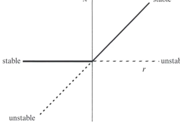
Saddle-Node Bifurcation
At the branch point r = 0, we find f′( x* ) = 0; the linearization disappears when the fixed points merge. Thus, points of intersection of the line and the curve correspond to fixed points for the system.
Transcritical Bifurcation
This equation defines a bifurcation curve in the ( a, b ) parameter space.) Next, find an approximate formula for the fixed point that bifurcates from x = 0, assuming that the parameters are close to the bifurcation curve. Then find new variables X and R so that the system reduces to the approximate normal form.
Laser Threshold
Assume that, in the absence of laser action, the pump keeps the number of excited atoms fixed at N0. Although this model correctly predicts the existence of a threshold, it ignores the dynamics of the excited atoms, the existence of spontaneous emission, and several other complications.

Pitchfork Bifurcation
For small x, the picture looks like Figure 3.4.6: the origin is locally stable for r 0, and two backward-bending branches of unstable fixed points split from the origin when r = 0. In the region rs r 0, two qualitatively different stable states coexist aside, namely the origin and the high-amplitude fixed points.
Overdamped Bead on a Rotating Hoop
Here’s the physical interpretation of the results: When H 1, the hoop is rotat- ing slowly and the centrifugal force is too weak to balance the force of gravity. In problems like this, it is helpful to express the equation in dimensionless form (at present, all the terms in (1) have the dimensions of force.) The advantage of a dimensionless formulation is that we know how to define small—it means "baie minder as 1." Verder, nie-dimensionalisering van die vergelyking verminder die aantal parameters deur hulle saam te voeg in dimensielose groepe.

Imperfect Bifurcations and Catastrophes
Saddle node bifurcations occur along the boundary of the regions except at the apex where we have a codimension-2 bifurcation. We choose the coordinates along the wire so that x = 0 occurs at the point closest to the bearing point of the spring; let a be the distance between this support point and the wire.
Insect Outbreak
To get rid of the parameters in the predatory term, we divide (1) by B and then let The complication is that these parameters can fluctuate. slowly as the state of the forest changes.
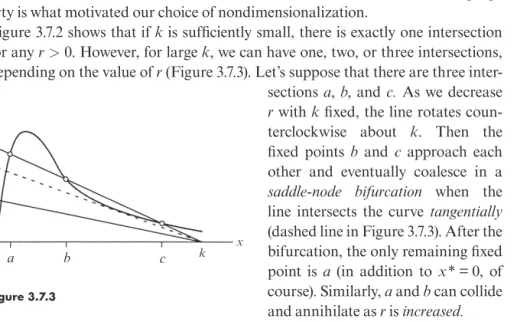
Saddle-Node Bifurcation
The experimental observations indicate that for a young forest, typically k x 300 and r 1 / 2 so the parameters lie in the bistable region. However, as the forest grows, S increases and therefore the point (k, r) drifts upwards in parameter space towards the outbreak region of Figure estimates that r x 1 for a fully mature forest, which lies dangerously in the outbreak region.
Transcritical Bifurcation
Laser Threshold
This procedure is often called adiabatic elimination, and the evolution of N(t) is said to depend on that of n(t). c) What type of branching occurs at the laser threshold PC. In the simplest case H1, H2 L; then P and D relax rapidly to stable values, and can therefore be eliminated adiabatically as follows.
Pitchfork Bifurcation
Consider the bead on a tilted wire discussed at the end of Section 3.6. a) Show that the equilibrium positions of the bead satisfy. Verify that this result reduces to the approximate result in part (d). g) Give a numerically accurate plot of the bifurcation curves in the ( r, h ) plane. h).
Insect Outbreak
Let G (t) denote the concentration of the gene product, and assume that the concentration S0 of S is fixed. Here A is the concentration of unphosphorylated protein and AP is the concentration of phosphorylated protein.
FLOWS ON THE CIRCLE
Introduction
Examples and Definitions
Explain why RR cannot be considered a vector field on a circle, for R in the range d R d. As we can, there is no way to consider RR as a smooth vector field over the entire circle.
Uniform Oscillator
Nonuniform Oscillator
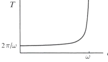
For an Now we want to derive a general scaling law for the time it takes to pass a bottleneck.
Overdamped Pendulum
To think about this problem physically, you have to imagine that a pendulum is immersed in molasses. If H is 1, the applied torque can never be balanced by the gravitational torque and the pendulum will keep tipping over.
Fireflies
Assume that R( )t is the phase of the firefly's flashing rhythm, where R 0 corresponds to the moment when a flash is emitted. As the phase difference approaches a constant, the firefly's rhythm is said to be phase-locked to the stimulus.
Superconducting Josephson Junctions
For each of the following vector fields, find and classify all the fixed points, and sketch the phase portrait on the circle. Instead of the two Josephson junctions in Figure 1, consider a series of N junctions in series.
Part II
TWO-DIMENSIONAL FLOWS
LINEAR SYSTEMS
Introduction
Definitions and Examples
But by the time the mass reaches is and v is zero again (Figure 5.1.4c).
Classification of Linear Systems
Solution: If the eigenvalues are complex, the fixed point is either a center (Figure 5.2.4a) or a spiral (Figure 5.2.4b). In our analysis of the general case, we have assumed that the eigenvalues are distinct.
Love Affairs
5.1.10 (Retraction and Liapunov Stable) Here are the formal definitions of the various types of stability. Be sure to show all the different cases that can occur, depending on the relative sizes of the parameters.
PHASE PLANE
Introduction
Phase Portraits
A direction field plot is clearer: short line segments are used to show the local flow direction. Even with the limited information obtained so far, Figure 6.1.3 gives a good understanding of the overall flow pattern.
Existence, Uniqueness, and Topological Consequences
In other words, the existence and uniqueness of solutions are guaranteed if f is continuously differentiable. From now on we will assume that all our vector fields are smooth enough to guarantee the existence and uniqueness of solutions starting from any point in phase space.
Fixed Points and Linearization
The answer is yes, as long as the fixed point for the linearized system is not one of the limiting cases discussed in section 5.2. The important Hartman-Grobman theorem states that the local phase portrait near a hyperbolic fixed point is “topologically equivalent” to the phase portrait of the linearization; in particular, the stability type of the fixed point is faithfully captured by the linearization.
Rabbits versus Sheep
Now we use common sense to fill in the rest of the phase portrait (Figure 6.4.6). For example, the basin of attraction for the node at (3, 0) consists of all the points that lie below the stable manifold of the saddle.
Conservative Systems
But note - the trajectories must maintain a constant altitude E, so that they run around the surface, not below it. Alternatively, there are counterexamples due to fixed points on the energy contour—see Exercise 6.5.12.
Reversible Systems
To show that the system is not conservative, it suffices to show that it has an attractive fixed point. The system in Example 6.6.3 is closely related to the model of two superconducting Josephson junctions connected by a resistive load (Tsang et al. 1991).
Pendulum
It also becomes clear that the saddle points in Figure 6.7.3 are all the same physical state (an inverted pendulum at rest). But if you think about the coordinate system shown in Figure 6.7.6, you will see that the picture is correct.
Index Theory
Then the index of the closed curve C with respect to the vector field f is defined as. If we reverse all the arrows in the vector field by changing t l t, the index does not change.
Theorem 6.8.2: Any closed orbit in the phase plane must enclose fixed points whose indices sum to 1
- Phase Portraits
- Existence, Uniqueness, and Topological Consequences
For each of the following systems, find the fixed points, classify them, sketch the neighboring orbits, and try to fill in the rest of the phase portrait. Sketch the phase portrait and thereby show that the fixed point r* 1, R* 0 attracts, but is not Liapunov stable.