The strength of the Big Bang theory is that it predicted large phenomena quite accurately before they were observed. This shift of the spectrum lines, due to the fact that galaxies are moving away from the observer, is called "redshift".

Big Bang Nucleosynthesis
Cosmic Microwave Background(CMB) Radiation
Friedmann Equations
Gravitational Instability and Structure Growth
- Linear perturbation theory and spherical collapse
- Cosmological N-Body Simulations
The gravitational pecular acceleration g is related to the gravitational potential Φ through the relation g = −∇αΦ, where α is the scale factor of the universe. In the case of dark matter and baryonic simulations, the representation of the density distribution becomes a more complicated task.

The Current Standard Cosmological Model
Large Scale Structure of the Universe
- Galaxies
- Clusters and Groups of Galaxies
- Superclusters: Clusters of Clusters
- Voids
The first, the CfA (Center for Astrophysics), provided the first discrete implication of the large-scale structure of the universe. The blurry picture of the structure of the universe became clearer as more redshift studies followed. The disk contains mainly younger stars, gas and dust and this is where the arms of the spiral galaxies are located.
The gas is trapped in the gravitational well of the dark matter, which is the dominant form of matter in the cluster. Other components of the cosmic foam are the plates or walls, which, as the name suggests, are thin (2D) formations. In Figure 2.15 you can see the large scale of the universe as constructed by the 2dF Galaxy survey.
The cosmic inventory has shown the existence of the fourth component of the Cosmos, the Voids.
Environment
- Structure finding- Web element characterisation
The 'percent rank' is the ranking of the specific object among the other objects in the catalog, i.e. Methods based on the topology of the cosmic web: Discrimination between different cosmic web patterns has been achieved by using topological methods. The use of the Minkowski functionals and especially the genus of the density field has proven to be a strong technique for distinguishing different patterns in space (Coles & Plionis, 1991; Mecke, Buchert & Wagner, 1994;).
A modern and quite effective approach is to classify the various cosmic web elements, based on the eigenvalues of the tidal tensor, the Hessian matrix of the Newtonian gravitational potential and written as Tij =∂i∂jϕ. Then, each point in space is geometrically classified as Void, Sheet, Filament, or Knot based on the number of eigenvalues of the tidal tensor that are above a given threshold value, λth. An alternative method is to use the velocity shear tensor instead of the tidal tensor.
An interesting method, the Multiscale Morphology filter, has been proposed by Aragon-Calvo et al. 2013), where the Hessian matrix method is used after applying smoothing kernels of different scales to construct the density field.

Halo Mass function
Although the choice of shear tensor can lead to more accurate discrimination at small scales, both techniques lead to similar results in linear theory. Furthermore, the latter technique is not suitable for use in redshift surveys, as the shear tensor cannot be observed, while the tidal tensor approach can still be used (Alonso et al., 2015). The vertical axis is the multiplicity function (M2ρ−1)(dn/dM), where ρ is the mean density of the universe.
The solid black lines are the analytical predictions using the fitted functional form proposed by Jenkins et al. 2001 ) and the blue dashed lines are the analytic predictions of the Press and Schechter (1974) analytic form (from Springel et al. 2005 ).

Aim of this Thesis
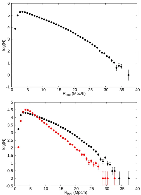
So the method of adaptive aperture is somehow a way to normalize density with the virilization properties of each halo. We chose to investigate the behavior of halo abundance function for isolated haloes and pairs of haloes and compare it with that of non-isolated ones. The criterion of isolation for both haloes and pairs of haloes is the isolation radius (Risol), that is, the distance from the halo or the pair's nearest neighbor.
Our method does not include any classification of web elements, but the way to define isolation is absolute and allows us to draw useful conclusions about the difference in abundance functions between extreme cases of Risol.
Simulation Data
General
Redshift & Projected Distributions
Definition of local environment
Lower panel: distribution of Risol for the 200K lowest (black) and highest mass (red) haloes of the light cone DM halo sample. The observed difference is expected as low-mass haloes more homogeneously populate both high- and low-density regions. This is quite an interesting fact, which can provide insight into the halo formation processes in extreme environments, and which we will study in more detail in a future study.
A final but important methodological issue is related to the fact that, by directly using the Risol parameter as a characterization of the local environment, we do not take into account the halo size, which inevitably affects the available minimum separation between haloes of different size. Therefore, in the remaining part we have chosen to use a parameterized characterization of the local environment provided by the isolation radius in units of the halovirial radius, that is, Risol/rvir. In addition to investigating the dependence of the abundance functions of haloes with different isolation status, we sought to extend our analysis to study the dynamics of isolated pairs.
We considered as pairs those haloes whose isolation radius Risol ranked among the 10% lower values of the entire dataset, and we calculated the second nearest neighbor for each central halo in the entire dataset.
Halo abundance function
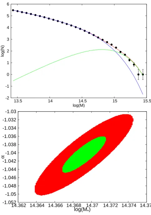
We first fit a single power-law function, such as Schether, and determine the best-fitting values of α, C1, and M⋆. We then fit the function as Schether with a double power law, but keeping the above three parameters constant at their best-fit first-step values, ie, allowing only C2 and β to be fit in this step both. If the reduced χ2 provided by the second step fit is lower than that of the first step, we consider that the double power law version of the Schether-like function is a better approximation to the abundance function of halo in the study.
The green line corresponds to the second power law fit, while the joint Schether function of the two power laws of equation (1) is shown as the red curve. The uncertainties of the α and M⋆ parameters in the first-step fit are calculated after marginalizing one over the other, keeping the normalization of C1 constant to the best-fit value. Although there is significant degeneracy of the parameter α, we see that the parameter M∗ is very well bounded with extremely small uncertainty.
The Schether-like analytic function, Φ(M), is represented by continuous curves. The single Schether power-law function is shown in blue, the double power-law function in red, while in purple we show the second power-law fit separately).
Results
- Nearest neighbour analysis
- Adjusting the definition of environment to the DM Halo’s physical dimensions
- Summary & Comparison of the two approaches
- Isolation status of pairs
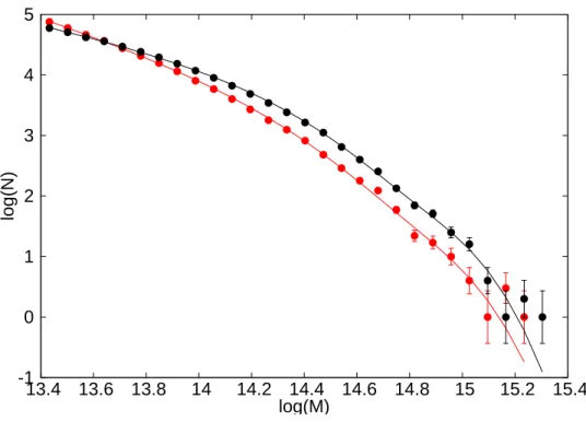
We quantify the behavior of the abundance function and its dependence on the environment using the two fitting parameters: that of the slope, α, and the characteristic mass, M⋆. Clearly, haloes of the same isolation state (same color in Figure 5.4) have similar AF and the difference between them is determined by the gravitational evolution, as one would expect. In this way we normalize the isolation criterion for the physical dimensions of the dark matter haloes.
Although we have a relatively small number of highly isolated haloes and thus statistically important uncertainties, the normalized AF for the two different isolation states shows significant differences for both redshift bins. As we have found in the corresponding Figure 5.4 in the previous analysis, the AFs with the same isolation status are similar, due to their differences due to gravitational evolution. We proceed to quantify such differences not only in the extreme isolation cases, but also for all different isolation statuses, by fitting the two parameters of the abundance-Schether-like function as a function of Risol/rvir, which we present in Figure 5.9.
We set the isolation radius Risol as an estimator of the local environment and we investigated the behavior of the AF for different isolation states as well as the redshift dependence of our results. Investigating the isolation status of pairs could be explored using the second nearest neighbor of the central halo. The behavior of the two fitted parameters, α and M⋆, with isolation, as defined by the two isolation distances (red), and compared to what we found previously using only Risol, as an estimator of the local environment (black), is presented in figure 5.13.
Conclusions
As expected, the number of haloes found in isolated regions is larger at high redshifts compared to low redshifts, while AF in most cases for haloes with the same isolation status, even if they have a similar shape, their differences are due to gravitational evolution; that is, however, we show that the high-redshift AF of highly isolated haloes unexpectedly exceeds the low-redshift, a result consistent with the upturn of M⋆ and the fact that this upturn originates at high redshifts. Therefore, we conclude that there must be a significant evolution of the isolation of the most massive isolated haloes, an interesting result that requires further investigation.
Finally, we would like to emphasize that an optimal and reliable environmental criterion is our monoparametric estimator, consisting of the normalized distance, (Risol/rvir), to the first neighbor. Uses as an additional parameter the distance to the second neighbor, (Risol2/rvir), to clearly identify high density areas corresponding to.
Appendices
This is the method we use in our analysis to find the best-fitting curves for abundance functions. In this section we present the basic principles of the method. Suppose we have a set of independent N measurements (xi, yi) of the quantity of interest y for a given xi and the error of the measurement is σ. The total measurement probability for the entire set of N experimental pairs (xi, yi) is equal to the product of the probabilities for each experimental measurement (C.Laub,T. Kuhl):
For a theoretical prediction expressed via a functional form f(xi,p), where the vectorp is a set of free parameters, we can obtain those values of the parametersp that minimize the χ2 term, thereby maximizing the total probability. Confidence intervals corresponding to a certain percentage of the probability distribution of parameters p are determined by limits of the quantity ∆χ2, based on the number of fitted parameters Nf 1. To estimate the extent to which the experimental values are fitted by the theoretical functional form we need calculate the reduced chi-square equal to χ2min divided by the degrees of freedom, χ2min/d.o.f.
For N number of experimental measurements and a number of Nf fitted parameters, the degree of freedom is given by the d.o.f.

Bibliography