The evolution of the XRF technique in the field of Cultural Heritage is also discussed. The third chapter catalogs the reference materials used for the experimental part of the project.
The role of XRF spectroscopy in Cultural Heritage scientific investigations . 2
Nowadays this can also be done by the Monte Carlo simulation programs, since in the last two cases a good calibration of the instrument is necessary (Galli & Bonizzoni, 2014). In the X-ray fluorescence (XRF) technique, an X-ray stimulating beam irradiates a multi-element sample by ionizing the inner atomic shells of the contained elements, thereby causing the emission of the corresponding characteristic X-rays.
Analytical methodology and expected results
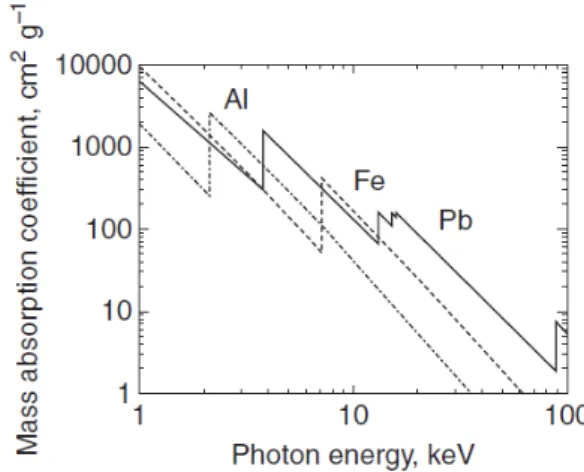
X-ray interactions with matter
The photoelectric absorption
When a bound electron reacts with a photon, the energy transferred is equal to the difference between the photon energy (Eo) and the binding energy (Ux) (Ζαρκάδας, 2001). The difference in wavelength of the incoming and outgoing photons can be calculated from Eq.
Emission of characteristic X-Rays
The energy of the emitted photon depends on the difference in the energy of the shell that lost the electron and that offered by the electron to fill the vacancy. The fluorescence yield depends on the atomic number of the element to which the atom belongs, but also on the shell in which the hole appears.

XRF instrumentation
The amount of these pairs is proportional to the energy of the X-ray photons. The height of the pulse produced is proportional to the energy of the respective incoming X-rays.

Historical evolution of the XRF analysis in the field of Cultural Heritage
The MCA memory is directed to the computer by means of an appropriate connection. With these, even today, the wavelength of the X-ray produced can be studied with high detection capability.
Description of the portable milli-probe XRF spectrometer
The silver alloys used were manufactured by the Institute of Nanostructured Materials, CNR, Research Area of Rome, Italy, within the framework of the PROMET (Protection of Metals) program “Developing new analytical techniques for monitoring and protecting metal artefacts from the Mediterranean region". According to the report of the Institute of Italy, pure copper, silver and lead in powder form were used as starting materials for the preparation. The electron backscattering technique showed that small accumulations of copper were formed in the alloys, because this element does not completely dissolve in silver.
More specifically, it has been proven that the solubility of copper in silver is 8-10% at 780 ° C resulting in the separation of these two metals and the formation of tree structures. Gold alloys, provided by Fischer-Helmut (www.fischer-technology.com), were developed as standard samples for application in X-ray micro-fluorescence (Helmut Fischer, 2012).

The Monte Carlo method
General
The basic idea of a general Monte Carlo simulation of ED–XRF spectrometers is to predict the response of X-ray and spectroscopy experiments. Monte Carlo can be used for optimization and design of experimental setups in silico, for dose calculation, estimation of detection limits and quantification.
The XMI-MSIM software package
In this interface you can define the position and orientation of the system of layers, detector and slits. Detector window normal vector: the detector window normal vector, which must be directed towards the sample. Active detector area: this corresponds to the area of the detector window capable of passing through detectable photons.
Detector zero: the energy of the first channel in the spectrum (channel number zero). Detector Fano factor: measure of the spread of a probability distribution of the fluctuation of an electric charge in the detector.

XRF spectrum analysis
General
In the batch simulation results window it is possible to analyze specific elements, lines, areas of interest, etc. Some of these are the photoelectric cross section, the secondary fluorescence effects, the matrix mass attenuation coefficient and the thickness of the sample. . The relationship between the intensity of an element and the composition of the sample is described by Sherman's mathematical equations.
1, where 𝜀𝜀𝑑𝑑(𝐸𝐸𝑖𝑖) is the intrinsic efficiency of the X-ray detector and φ2 is the angle between the detector and the sample surface. Another point of interest in qualitative and quantitative XRF analysis is the correct estimation of the spectral background to obtain accurate net count rates.

The PyMca software toolkit for XRF spectrum analysis
Matrix effects causing secondary fluorescence, cascade effects and scattering of both primary and secondary fluorescence radiation can lead to an overestimation or underestimation of the concentration and the quantitative analysis can become much more complicated (Polese, 2015). Various parameters can be defined in the configuration window of the Advanced Fitting interface, such as the area to fit, escape, accumulate, spread peaks, the fitting function, the shape of the peak. The absorbers, matrix composition, source and detector parameters can also be defined here.
The incident beam flux, which is one of the basic parameters since the fluorescence line intensities are linearly proportional to its value, can be defined in the Concentrations tab. By using the right configuration file, depending on the analysis case, one can fit the peaks of interest and obtain results on the net peak areas and concentrations of the sample constituents.
Characterization of the pXRF spectrometer
- High voltage setting
- Tube current linearity
- Filters characterization in the excitation channel
- Thickness of the X-ray detector crystal
- Energy distribution of the X-ray tube excitation spectrum
The branching ratio Kβ/Kα of relative radiative transition probabilities was calculated based on the xraylib database (Schoonjans, n.d.). Experimental intensity ratio (𝚰𝚰𝑲𝑲𝜷𝜷 . 𝑰𝑰𝑲𝑲𝜶𝜶) (asterisks in the graph) and their theoretical calculations (lines in the graph) for different crystal thicknesses. The ratio of the experimentally measured continuum over the simulated one is presented in Figure 1.
Polynomial fit to the experimental over simulated relationship of the intensity of the continuum distri-. Linear fits to the experimental over simulated relationship of the intensity of the continuum distribution (13-32 keV).

Comparison between pXRF measurements and MC simulations (charts,
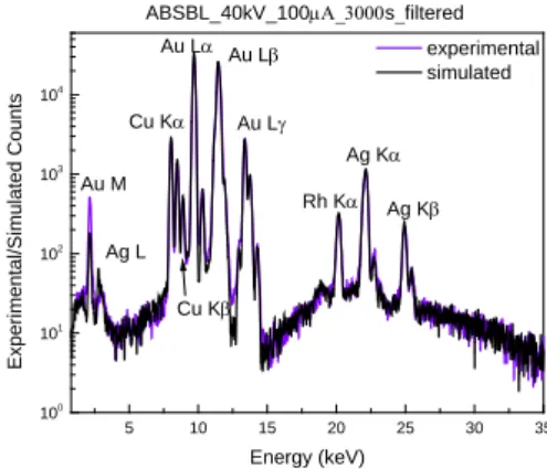
Gold alloys
The following graph presents the % difference between experimental and simulated net peak area intensities of the detected characteristic X-ray lines as extracted by means of the PyMca Toolkit. The % difference between experimental and simulated net peak area intensities of the detected characteristic X-ray lines of gold alloys.
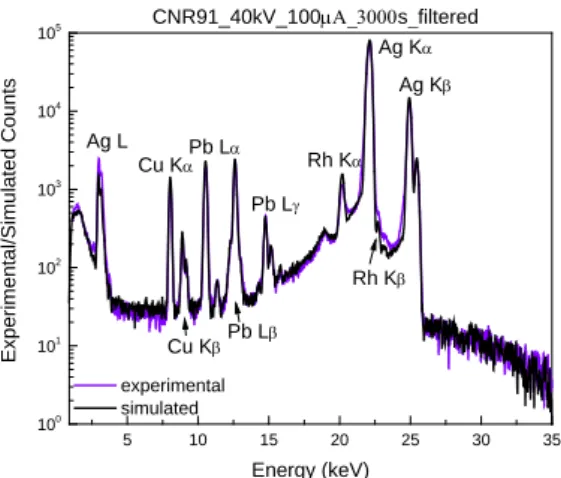
Silver alloys
The % difference between experimental and simulated net peak area intensities of the detected characteristic X-ray lines of silver alloys. In silver alloys, the Ag is the predominant component and the Ag-Kα lines are accurately simulated with differences below ~6% between the experimental and simulated intensities. In CNR-91, where the Cu concentration is 1.5%, the Cu-Kα intensity is overestimated by ~21%, while for other concentrations the observed differences are less than ~5%.
The observed deviation for Cu-Kα intensity for the reference silver alloy CNR-91 could be attributed to the possible inhomogeneity of Cu distribution within the alloy.
Copper alloys
The % difference between experimental and simulated net peak area intensities of the detected characteristic X-ray lines of copper alloys. The elements Zn and As were analyzed and compared by their respective Kβ lines in order to avoid systematic errors in the analysis of their Kα peak areas due to spectral interferences (Cu-Kβ with Zn-Kα and As-Kα with Pb-La ). In the cases where the concentration of both elements is below 1% (close to detection limits), the experimental measurements significantly overestimated the simulated counts by ~50-54% for Zn and.

Discussion
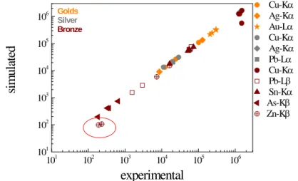
A comparison between the simulated versus experimental peak counts obtained from the analysis of the various reference gold, silver and copper alloys. The present study proposed a universal way to optimize the description of tube emission spectrum without requiring dedicated setup for direct measurements of the tube emission spectrum. The comparison of simulated and experimental characteristic X-ray net peak area intensities showed differences that are less than about ~20% for major and minor elements in gold, silver, and copper alloys.
More specifically, the simulated peak areas of Au-Lα, Ag-Κα and Cu-Kα (in gold alloys), Ag-Kα, Cu-Kα and Pb-Lα (in silver alloys) and Cu-Kα, Sn-Kα are Pb-Lα (in copper alloys) systematically higher, up to 10%, compared to the experimental one. This fact strongly suggests that these differences could arise from a slight (several percent) underestimation of the geometric parameters responsible for incident and detection solid angle calculations.
Introduction (gold, silver, copper)
However, it is not so dangerous because it is possible to calculate its results and the life of the metal. Tarnishing (dark colored copper sulphides) occurs as a result of the reaction between copper and sulfur in the air. When fresh copper alloys are exposed to air, corrosion due to water-soluble corrosion projects rapidly spreads, resulting in the formation of green spots on the adjacent surface.
Stress corrosion cracking or uniform corrosion can be caused to copper alloys due to ammonia, through the formation of soluble complexes with copper and copper ions. Galvanic corrosion can occur in copper alloys when they come into contact with other metals or fasteners (Selwyn, 2004).
Monte Carlo simulations of corroded metallic alloys
Gold alloys
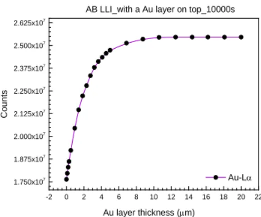
The variation of the Cu-Ka counts with respect to the thickness of a surface enriched in pure gold. The variation of the Au-M counts with respect to the thickness of a surface enriched in pure gold. The variation of the Au-Lα counts with respect to the thickness of a surface enriched pure gold.
Variation of the Au-Lα/Αu-M intensity ratio with respect to the thickness of an enriched surface. The variation of Ag-Kα is calculated relative to the thickness of an enriched pure gold surface.
Silver alloys
Copper alloys
The variation of Sn-Kα is calculated in relation to the thickness of the cassiterite layer formed on the over-. The variation of Sn-Lα is calculated in relation to the thickness of the cassiterite layer formed on the over-. The variation of Cu-Kα is calculated in relation to the thickness of the cuprite layer formed on the reference surface.
The variation of Sn-Kα is calculated in relation to the thickness of the cuprite layer formed on the reference surface. The variation of Sn-Lα is calculated with respect to the thickness of the cuprite layer formed on the reference surface.
