In the first case, we used a magnetized medium (plasma) within a non-magnetized FRW background model, and our results showed that the magnetic field did not affect the inflow velocity. The existence of magnetic fields in galaxies and clusters is something that has been proven through many observations in recent years. The effects of the magnetic field were now apparent, and our solution showed that the magnetic pressure added to the total pressure tended to slow the collapse of the fluid.
Fluid dynamics
The basic hydrodynamic equations that we will use are the continuity equations and the Navier-Stokes equations. For a self-gravitating, perfect fluid in the dust period (Newtonian limit), the continuity and Navier-Stokes equations take the form Our basic parameters are the density of the substance ρ, the pressure and the velocity of the fluid u, which means that we need an additional equation to close our system.
Fluid kinematics
Ohm’s law
One of the most important relationships in the field of electrical circuits is Ohm's law. ς in (21) is called conductivity and its value depends on the properties of the substance. The form of equation (21) is not yet complete, as the medium in our research moves with speed ua in the external magnetic field Ba.
This results in the appearance of the Lorentz force, which will act on electric charges. Ja =ς(Ea+abcubBc) (22) In this study, as we said, we will work with a perfectly conducting liquid. ς → ∞), which means that if we solve equation (22) for the electric field, we get the following expression for Ohm's law. 6electromotive force can be described as the electromagnetic work transferred to an electric charge due to the forces acting on the latter.
Ideal MHD
Magnetic evolution
What this really means is that regions of higher magnetic pressure exert a force towards regions of lower magnetic pressure.
Lorentz force
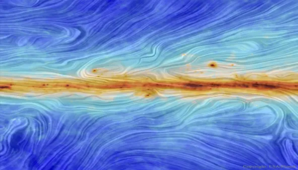
Everything we have said so far, as well as the set of equations we have extracted, in combination with the kinematic equations and constraints, monitor the evolution of a magnetized fluid in the Newtonian limit in general. In the first images of the CMB radiation we observed such disturbances in the temperature and, as a result, in the density distribution of the matter. In other words, there were areas in the early universe that were denser and other areas that were less dense.
According to the theory of gravitational instability, regions with too much density tend to collapse under their own gravity and become even denser, leading to the formation of stars and galaxies, while regions with too little density tend to drift apart and create the voids you observe today . So, if we want to make the FRW model more realistic and closer to the real image of the universe, we have to perturb it. In the first case (Section 5), we study the evolution of a magnetized fluid within a non-magnetized FRW model, while in the second case (Section 6) we decide to also include a background magnetic field to enhance its effects.
We choose to work in the dust era, where we have p = 0 and using Newtonian physics is an acceptable approximation. What is more, the integration of equation (41) leads us to the Newtonian form of Friedmann's first equation. So if we solve (44) for the scale factor, we get a ∝ t2/3 which corresponds to the Einstein-de Sitter model.
According to the above, in our study, the scalar quantities present in the background model are the density ρ and Θ that monitor the expansion/contraction of our fluid.
The new variables
Non-linear equations
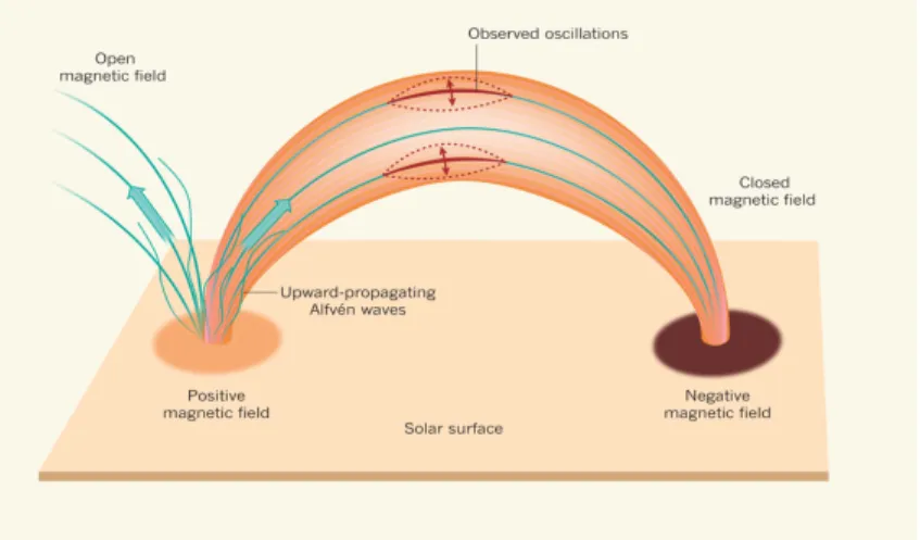
Similarly, we take the convective derivative of Ba, combine it with the evolution of the magnetic pressure (37) and end up with. Alv´en waves correspond to the oscillations of the ions that move through the liquid and the magnetic field. As we can see in figure 6, Alv´en waves propagate along the magnetic field (¯k//B), but the movement of the ions is perpendicular to B.
The first corresponds to the isotropic magnetic pressure and the other three are due to the tension of the magnetic field lines. Equation (53) gives us a lot of useful information about the behavior of our fluid and how the magnetic field affects it. What is more, the negative sign in front of Ba proves that any increase in the magnetic pressure (Ba > 0) works against the expansion of the liquid and in favor of the gravity of the substance.
This 'conflict' between σB2, ωB2 and σ2, ω2 arises as a result of the magnetic tension of the field lines. The latter is the cause that leads to the occurrence of magnetic shear and vorticity, which in turn oppose anything that tries to disturb the equilibrium of the field lines. On the other hand, the kinematic constraints we derived in section 2.2 do not contain magnetic terms, meaning that they are not directly affected by the presence of the magnetic field.
To be more precise, the fourth term in the right-hand side of equation (54) shows the effect of the magnetic pressure, while all the other terms containing the magnetic field appear due to the magnetic tension.
Linearisation
Finally, comparing the magnetic displacement σB2 and the vorticity ωB2 with their kinematic analogues, we note that the former is opposed to the latter. For example, as ω2 tries to rotate the medium and twist the lines of force, the magnetic tension reacts through ωB2, which tries to slow the rotation. Magnetic terms also appear in the convective derivatives of the other two (˙σab,ω˙a) kinematic quantities.
However, in this study we will not need any of them, so we choose not to mention them. Having rewritten the Navier-Stokes and Raychauduri equations, we can now take the convective derivative of Za. To obtain the final equation, we used equation (53), the trace of (52), as well as the convective derivative and spatial gradients.
The problem with this set of equations is that it is very difficult to solve.
Linear equations
Solving the system
We take yet another convective derivative of ∆ and end up with the following third-order equation. For the convective derivative in the last term of the equation above, we have n. 63) (see Appendix. Integrating the latter we obtain the relation that describes the density variations with respect to time, ρ=ρ0(a0/a)3, which we can replace in equation (68).
Harmonic decomposition
Jeans length and mass
There is a critical wavelength that separates stable from unstable gravitational variations and this is the Jeans length. 76) We get an increase in gravitational disturbances when λ >> λJ. In the case of disturbances with a wavelength smaller than the Jeans length, the pressure does not allow their increase. Specifically, the mass of Jeans corresponds to the mass of a sphere whose diameter is equal to the length of Jeans.
Zero-pressure scenario
In the previous section we studied the evolution of a magnetized, self-attracting fluid on a non-magnetized background. Here we are going to repeat the work we did in section 5, but now we will allow for the existence of a magnetic field in the background model. We assume that the Ba field is completely random so that it does not affect the homogeneity and isotropy of our fluid and hBai = 0, but hB2i 6 = 0, which means that the magnetic field contributes to the total energy of our system .
As in Section 5.1, we should first of all set our to our zero-order solution, which will play the role of our background later. These results show that the magnetic pressure decreases faster than the matter density.
The new variables (II)
Non-linear equations (II)
Specifically, any increase in ∆a or Ba slows down the expansion of our fluid (demonstrated by the negative signs in front of them), while the shear and vorticity of the magnetic field, σ2B, ωB2, act in opposition to the shear and vorticity of the fluid, σ2. , ω2 (ω2 tends to rotate the medium, while ωB2 tries to inhibit the rotation).
Linear equations
Solving the system (II)
Harmonic decomposition (II)
Zero-pressure scenario (II)
This result proves that the introduction of the background magnetic field made it strong enough, and as a result the magnetic effect began to show itself both in quantity and quality. First in quality, because the magnetic pressure was now included in our equations and, as we can see from equation (103), it affects the collapse speed of our liquid in a decelerating way. Secondly, in quantity, because through relation (104) we have a connection between the magnetic pressure, the wavelength and the effect they cause.
To be more specific, the higher the magnetic pressure c2a, the higher the value of A and, as a result, the greater the deceleration caused to ∆n. So the deceleration of ∆ is proportional to the magnetic pressure and inversely proportional to the wavelength of the disturbance. If this is indeed the case, then it is safe to wonder if the magnetic fields participated in the process that led to the formation of the structure we observe today. In this work, we studied two cases of Newtonian magnetized fluids collapsing inside an FRW background model.
This led us to the second example, where we tried to increase the effects of the B-field by introducing a magnetic field in our background as well (this added to the total pressure of our system, but was random in direction, so it did not affect the isotropicity of our background). Thus, after linearization with respect to the new background, we solved our system and the solution we got was quite different from the first case. Now our solution included the magnetic pressure and the perturbation wavelength, in contrast to the first case where the solution contained no pressure and was independent of wavelength.
Furthermore, we found that magnetic pressure tends to slow down the collapse rate of our fluid and the stronger the magnetic field is, the greater the slowdown becomes. On the other hand, the wavelength of the disturbance was inversely proportional to the delay and for very large wavelengths the effects of the magnetic field disappear and we return to the standard solution. If we go to the second derivative on the left of (109), we split it into two terms.