EXTENDED THEORY AND APPLICATIONS FOR EFFECTIVE DETERMINATION OF THE BRAIN ACTIVATED STATES IN

1, when noise was added to the sensor measurements as a percentage of the true values. In both cases the maximum high-frequency amplitude occurs in the descending phases of the low-frequency oscillations.

Introduction

INTRODUCTION 2

INTRODUCTION 3

INTRODUCTION 4

INTRODUCTION 5

Outline

INTRODUCTION 6

INTRODUCTION 7

Contributions

EEG measures the potential of this field on the surface of the head, in the form of voltage differences. To solve it, we need to impose modeling constraints and include prior assumptions about the resources in the model.

BASICS OF EEG-BASED BRAIN IMAGING 9

Anatomy of the Human Brain

BASICS OF EEG-BASED BRAIN IMAGING 10

Neuron Structure and Function

BASICS OF EEG-BASED BRAIN IMAGING 11

BASICS OF EEG-BASED BRAIN IMAGING 12

Electromagnetic Signal Generation and Mod- elling

BASICS OF EEG-BASED BRAIN IMAGING 13

BASICS OF EEG-BASED BRAIN IMAGING 14

The Forward EEG Problem

Head Models

The Inverse EEG Problem

Parametric Methods

BASICS OF EEG-BASED BRAIN IMAGING 17

BASICS OF EEG-BASED BRAIN IMAGING 18

Imaging Methods

BASICS OF EEG-BASED BRAIN IMAGING 19

BASICS OF EEG-BASED BRAIN IMAGING 21

EEG Recording Systems

EGI 300 Geodesic System

BASICS OF EEG-BASED BRAIN IMAGING 23

BASICS OF EEG-BASED BRAIN IMAGING 24

Event-Related Potentials

Conclusions

BASICS OF EEG-BASED BRAIN IMAGING 26

BASICS OF EEG-BASED BRAIN IMAGING 27

Introduction

The roots of the mathematical foundations for tomography lie in the groundbreaking work of Radon, who showed that every two-dimensional object can be uniquely reconstructed using line integrals [180]. VFT presents methods for vector field reconstruction using integral data over field projections in different directions. Previously, Juhlin outlined a model for recovering the solenoidal part of a divergence-free three-dimensional fluid field when certain values of the boundary field are known [101], which was later developed by Sparr et al.

In particular, the method proposes the discretization of a square-bounded domain in tiles and the reconstruction of the vector field at specific sampling points, which are the centers of the tiles. Ideal point sensors are placed in the middle of the outer edges of the boundary tiles. Thus, integral data can be considered as weighted sums of Cartesian components of a local vector field.

Thus, dense and uniform sampling of the Radon parameters, prerequisites for accurate image reconstruction, has been achieved.

The Proposed Scheme

Physical Model
Methodology Implementation
Ill-conditioning and Regularization via Discretization
Upper Bound in the Solution Error

Vector r indicates the direction vector of the line, while φ and θ are the azimuthal and polar angles, respectively. The coordinates of the generated points along the line increase incrementally in the three directions. An example of the sampling process along the line L and the assignment of the discrete line points to the centers of the tiles is shown in Fig.

When the same problem is formulated in the continuous domain, i.e., reconstruction is not implemented using sampling along the trace lines, the irrotational property of the vector field suggests that the line integral IL is equal to zero for a closed loop. An indicator of the bad state of the system is the state number of the transfer matrix K. The first approximation error is the result of the sampling operation, i.e., the mapping of points along the tracing lines to the nearest reconstruction points. .

The restoration of the field after the estimation of the coefficients of the system is carried out using the method of least squares.

Figure 3.1: A bounded cubic domain with edges length equal to 2U , discretized into tiles of size [P × P × P ]

Method Evaluation

Simulations on Electric Fields
Noise Effect Assessment
Comparison with Alternative Methods

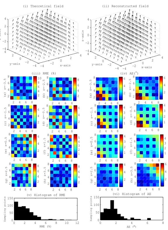
The error in the orientation of the field is smaller, still indicating the locations of the sources. Depending on the application, another natural noise source could be the movement of the sensors. The sensitivity of the method to the additive noise is high, especially when ∆r is small, confirming the intrinsic instability in this case.

Although the magnitude errors are not very small, field maxima larger than ∆r help determine the location of the source. 3.10(i),(ii)-(a):(d), in the case of perturbations in measurements and sensor positions (Simulation #3), the solution errors appear to be the accumulated error of the two previous cases. However, the model equations used can be used to recover the irrotational fields and within the geometric model described in this work.

A more detailed description of the ART implementation for comparison with 3D-VFT is provided in Appendix A.

Concluding Remarks

This is quite encouraging, given that some of the noise in the measurements can be handled using filtering techniques. After presenting the theoretical framework for the reconstruction of electric fields, we will focus on the application of the method to the inverse EEG problem. In both cases, (a)-(h) show the errors plotted on a part of the z-axis, for better visibility.

Finally, (v) and (vi) present the distributions of the two types of errors, i.e. RME (%) and AE (◦), respectively indicated in the corresponding figure legend. In both cases, (a):(d) present the errors when different percentages of sensors are disturbed, starting from 25% of the sensors and ending with their total. Consequently, the line integral between two sensors can be written as the difference of the potential values measured at the sensors.

Then we can define the regions of activation as the locations of high values of the reconstructed electric field.

Figure 3.4: A simulation example for the recovery of an electrostatic field, caused by a point source located at (15, 15, 15)

3D-VFT FOR THE INVERSE EEG PROBLEM 59

Adjustment of 3D-VFT for the realistic EEG inverse problem

3D-VFT FOR THE INVERSE EEG PROBLEM 60

3D-VFT FOR THE INVERSE EEG PROBLEM 61

Implementation within Brainstorm

3D-VFT FOR THE INVERSE EEG PROBLEM 62

3D-VFT FOR THE INVERSE EEG PROBLEM 64

Evaluation of the Method

Real Data

3D-VFT FOR THE INVERSE EEG PROBLEM 66

3D-VFT FOR THE INVERSE EEG PROBLEM 67

Simulations

3D-VFT FOR THE INVERSE EEG PROBLEM 68

3D-VFT FOR THE INVERSE EEG PROBLEM 69

Concluding Remarks

3D-VFT FOR THE INVERSE EEG PROBLEM 70

3D-VFT FOR THE INVERSE EEG PROBLEM 74

Different types of biomarkers, e.g. biochemical, genetic, neuroimaging and physiological, have been proposed to diagnose Alzheimer's disease (AD), the most common cause of dementia, and mild cognitive impairment (MCI), a neuropathology that does. not noticeably affect cognitive functions. ERP methods provide a non-invasive, inexpensive means of analysis and have been proposed as sensitive biomarkers of cognitive impairment; furthermore, different ERP components are strongly associated with working memory, attention, sensory processing, and motor responses. In this chapter, we use an auditory oddball task and we record high-density EEG data from healthy elderly controls, MCI and AD patients.

The MMN and P300 ERP components are then extracted and examined for their association with neurodegeneration. The results presented in this chapter are a joint work with Vasiliki Kosmidou and Anthoula Tsolaki.

AUDITORY MMN AND P300 IN MCI AND AD 77

Introduction

AUDITORY MMN AND P300 IN MCI AND AD 78

AUDITORY MMN AND P300 IN MCI AND AD 80

Materials and Methods

Experimental Issues
Implementation Issues

Results

Behavioural Results

ERP analysis

AUDITORY MMN AND P300 IN MCI AND AD 83

AUDITORY MMN AND P300 IN MCI AND AD 85

Active Brain Areas Analysis

AUDITORY MMN AND P300 IN MCI AND AD 86

AUDITORY MMN AND P300 IN MCI AND AD 87

Discussion

AUDITORY MMN AND P300 IN MCI AND AD 88

AUDITORY MMN AND P300 IN MCI AND AD 92

Conclusions

In this chapter, we recorded high-density EEG data while presenting pictures of two classes of facial affect, i.e., anger and fear, to young and elderly participants. We then used 3D-VFT to map the activated states of the brain at the N170 ERP component, at relevant regions of interest. The results showed that the elderly showed larger N170 amplitudes, while age-based differences were also observed in the topographic distribution of the EEG recordings at the N170 component.

The results on the maximum activation area appeared to be emotion specific for the group of young people. These findings may indicate that older adults use more resources to regulate negative emotions, and that the regulatory mechanisms for the two emotions are similar.

AGE EFFECT ON EMOTION MECHANISMS 95

Introduction

AGE EFFECT ON EMOTION MECHANISMS 96

Participants
Emotional Stimuli

Implementation Issues

Results

EEG Analysis
Active Brain Areas Analysis

AGE EFFECT ON EMOTION MECHANISMS 99

AGE EFFECT ON EMOTION MECHANISMS 102

Discussion

AGE EFFECT ON EMOTION MECHANISMS 103

AGE EFFECT ON EMOTION MECHANISMS 107

Conclusions

The effect of gender on rapidly allocating attention to objects, features, or locations, as reflected in brain activity, is examined in this chapter. During the task, high-density EEG data were recorded and analyzed using behavioral ERPs, i.e. The P300 component and neural analysis using 3D-VFT. Twenty subjects (half female; 32±4.7 years) participated in the experiments and performed 60 trials for each condition.

Behavioral analysis showed that both women and men performed better in the pop-out condition compared to the search condition in terms of accuracy and reaction time, while no gender-related statistically significant differences were found. Nevertheless, in the search condition, higher P300 amplitudes were detected for females compared to males (p

The results presented in this chapter are joint work with Vasiliki Kosmidou and Katerina Adam.

GENDER EFFECT IN ATTENTION MECHANISMS 109

Introduction

GENDER EFFECT IN ATTENTION MECHANISMS 110

Participants

Behavioral task

Implementation Issues

Results

Behavioral Results
ERP Results

Brain Source Results

Concluding Remarks

GENDER EFFECT IN ATTENTION MECHANISMS 115

GENDER EFFECT IN ATTENTION MECHANISMS 118

Recent evidence suggests that cross-frequency coupling (CFC) plays an essential role in multi-scale communication across the brain. The amplitude of the high-frequency oscillations, responsible for local activity, is modulated by the phase of the lower-frequency activity, in a task- and region-relevant manner. We identify the lower frequency components that contribute more to the conditioning of the high frequency activity across the whole brain and we further investigate their differentiation according to the experimental task's variation.

To measure PAC, we use the GLM measure that has been shown to work well for short-length data as implemented in [69], and then we conduct a case study using event-related PAC (ERPAC), which is more suitable to capture PAC in event-related datasets. Stronger coupling was observed in the delta band, which is closely associated with sensory processing.

3D-VFT BASED AUDITORY PAC 120

Introduction

3D-VFT BASED AUDITORY PAC 121

Data Acquisition and Preprocessing
Phase-Amplitude Coupling

3D-VFT BASED AUDITORY PAC 122

3D-VFT BASED AUDITORY PAC 123

Event-Related Phase-Amplitude Coupling

Results

3D-VFT BASED AUDITORY PAC 125

3D-VFT BASED AUDITORY PAC 127

ERPAC

Concluding Remarks

3D-VFT BASED AUDITORY PAC 133

The aim of this thesis was to present an alternative methodology for solving the inverse EEG problem and apply it towards advancing the state of the art in cognitive research. Current methods that attempt to estimate neural activity from EEG recordings model neural sources as dipoles and solve the forward problem, for which they must model scalp properties and bioelectric field propagation. The main drawback of these methods is that the conductivity properties of the medium through which the fields propagate are not known, and inaccurate modeling can severely affect the solution of the forward problem.

In this thesis, instead of using source and volume conduction modeling, we proposed to reconstruct the electric vector field inside the head. However, due to the use of line integrals, we do not need to know the conductivity of the tissues inside the head, nor the underlying source model. First, we developed a method (3D-VFT) for the numerical reconstruction of 3D, continuous, irrotational vector fields in a bounded domain, which are properties that bioelectric fields have inside the head.

When the vector fields are caused by sources within the domain, the maxima of the fields can determine the location of the sources.

CONCLUSIONS AND FUTURE WORK 135

CONCLUSIONS AND FUTURE WORK 136

CONCLUSIONS AND FUTURE WORK 137

CONCLUSIONS AND FUTURE WORK 138

The reconstruction proposed in [221] which is based on the Algebraic Reconstruction technique (ART) suggests the discretization of the bounded field domain and considers the line integrals connecting boundary points that are known. Here, the linear system is formulated by calculating the lengths of the line segments that lie within each crossed tile u. In particular, if Ih, fu, rh and kh, u is used to denote the line integral of the tracing line Lh, the unknown field value in tile u, the direction vector of the line, and the length of the line Lh inside the tileu , respectively, then each of the system's equation will have the form

ART was implemented in this thesis considering the limited domain and sensors used for the development of 3D-VFT. The irrotational property still allows the calculation of ILh from the difference of the values measured at the two boundary points. After discretizing the region on a three-dimensional cubic grid, with grid steps ∆x= ∆y= ∆z = ∆P, the central difference (or finite difference, since ∆P is considered to be finite) to approximate the derivative the second at a point [i, j, k] with respect to x is.

This method was applied to the geometric model used for the development of 3D-VFT to reconstruct irrotational fields and compare the methods.