Graphene and Monolayer hBN Using Equilibrium Molecular Dynamics

Introduction: Graphene and hBN

Discovery and Unique Properties

Although theoretical predictions for the electronic band structure of graphene (in the form of graphite) were published as early as 1947 [1], theoretical studies on graphene and 2D materials generally remained only paper exercises until the first isolation and experimental observation of monolayer graphene by A. Borov nitride, on the other hand, although it has the same crystal lattice as graphene and has many of the same properties, is an insulator with a band gap close to 6 eV, making it an ideal dielectric substrate for graphene and MoS2 van der Waals heterostructures [8].

Electronic Band Structure

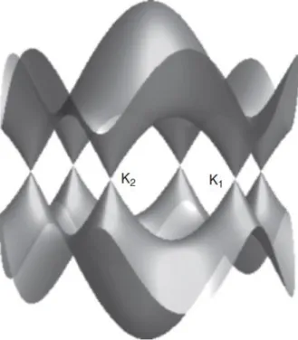
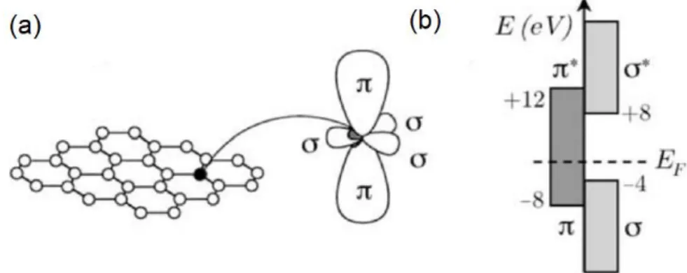
Here we are interested in shallow valence states near the Fermi level, so our treatment of tight bonding will only be concerned with π-bonding states formed by overlapping 2pz orbitals. The resulting energy surface of the band structure obtained from the tight-binding approximation through solution (15) is shown in Figure 5 .

Phonons in graphene and hBN

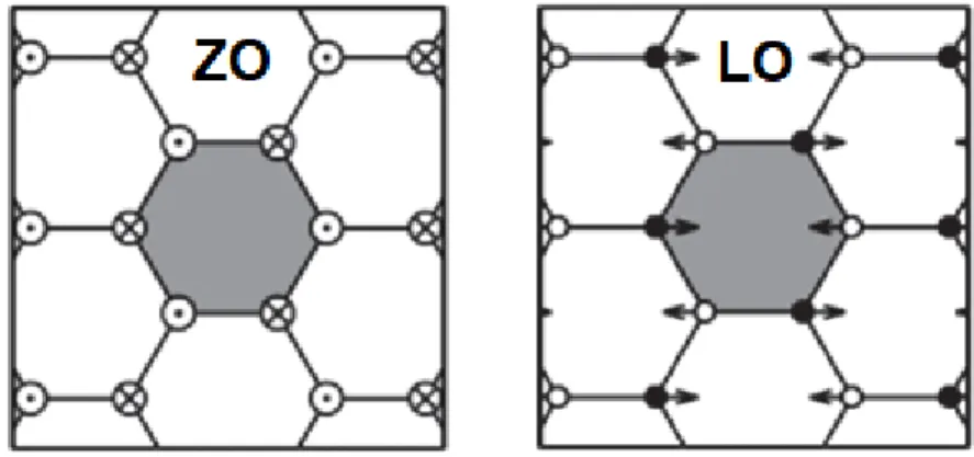
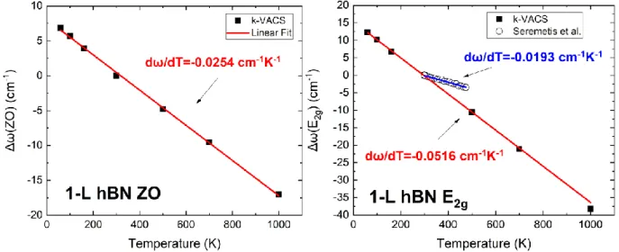
The central quantity of the method is the velocity autocorrelation sequence (k-VACS), denoted by 𝑍𝑥𝑝(𝒌, 𝑡𝑖) and given by the expression. Figure 30 also presents the temperature dependence of the ZO and E2g modes for graphene.

Molecular Dynamics Simulations

Introduction

This approach famously fails in the case of the description of the hydrogen bond, which is a purely quantum mechanical phenomenon. However, unless the boundary atoms are a small fraction of the atoms in the bulk of the system, boundary conditions can introduce significant computational artifacts.

Numerical Integration Algorithms: The Velocity-Verlet Algorithm

Considering that the simulation time steps must be smaller than the smallest time period of the vibrating component of the system in order to properly investigate its dynamics, typical time steps used are of the order of 1 fs, which would states that such simulations must be run for several hundred billion time steps. An alternative formulation of the Verlet algorithm, called the Velocity-Verlet algorithm, is the most widely used integrator in MD simulations, mainly because although it has the same accuracy and global errors for positions and velocities as the standard form, it has superior numerical. robustness with respect to floating-point arithmetic errors.

Simulating constant temperature (NVT) systems: The Nosé-Hoover thermostat

Applying Hamilton's equations of motion to the Hamiltonian (37), the differential equations for the system become. Furthermore, it is the same for all particles at any instant of time and directly models the interaction with the heat bath. The system (𝒓̅, 𝒑̅, 𝑠, 𝑝𝑠) (including the heat bath degrees of freedom) is a closed system and is therefore described by a microcanonical partition function.

Empirical Forcefield Potentials: The Tersoff-2010 Potential

Despite the simplicity of the potential, it can accurately predict the physical properties of liquid Ar by simple fine-tuning of the two potential parameters. The parameters 𝑅 and 𝐷 are chosen to include only the first neighboring shell of the central atom in the bonding interaction. In a similar previous work [46], it was shown that the LCBOP and AIREBO potentials [47] give a very poor description of the temperature dependence of the Raman active phonon energy E2g for graphene, which is the main subject of this work.

System Realizations and Case Studies

On the other hand, the width of the peak corresponding to the phonon decay rate must be obtained by fitting to Lorentzian functions. The phonon lifetimes of the zone-center states in the graph across the temperature range are shown in Figure 33. In Figure 34, we present the temperature dependence of the zone-center phonon decay rates in hBN.

The k-space Velocity Auto-Correlation Sequence Method (k-VACS)

Introduction to time-correlation functions

In the general case, suppose that the system is coupled to the external probe by a general interaction Hamiltonian given by [56]. The ensemble mean is taken with respect to the equilibrium distribution, although the system is not actually in an equilibrium state, due to the external perturbation. 𝐴(𝒌, 𝜔)〉 = χ𝐴𝐵(𝒌, 𝜔) ∙ 𝐹(𝒌, 𝜔) (58) This is the well-known result of linear response theory, namely that the macroscopic effect of the external system is linear disturbance.

The k-VACS method

This is a direct consequence of the definition of the equilibrium position, since the time-averaged displacement of an atom from its equilibrium position must be zero. Another quantity that will later play a major role in our attempt to extract phonon energies and lifetimes is the Fourier transform of the k-VACS, namely. This is a direct consequence of the complexity and chaotic nature of dynamical systems with many degrees of freedom and complex dynamics, such as macroscopic physical systems.

Extracting phonon energies and lifetimes

We will now attempt a rough sketch of the proof, but first we need the definition of Power Spectral Density (PSD), which is given by the relation. Also by the definition of the normal mode coordinates and the space-time Fourier transformed velocities in the frequency domain we have. where the dot indicates the derivative with respect to time. This is exactly the statement that we wanted to prove, namely that the total Power Spectral Density of the velocities in (𝒌, 𝜔) space is a linear superposition of Lorentzian peaks, centered at the anharmonic phonon eigenfrequencies and with half-widths at -half maximum equal to the decay constants 𝛤(𝒌, 𝑗), which are directly related to the lifetimes via Eq.

The Projected Density of States

In the framework of the pure Green's Functions formalism, each Lorentzian peak is a superposition of δ functions at each point of the peak; the fully interacting system then has a continuum of stationary energy eigenstates around the center of the vertex. The idea of ​​a phonon lifetime arises when we look at the continuum of eigenfrequencies of the interacting system around the center of the tip as a central "quasi-phonon" that has uncertainty in its energy; by Heisenberg's Uncertainty principle, this translates directly into a finite lifetime for this renormalized anharmonic phonon. Quantity | ______(𝑝|𝒌, 𝑗)| PDOS) of atomic species 𝑝 in the total DOS.

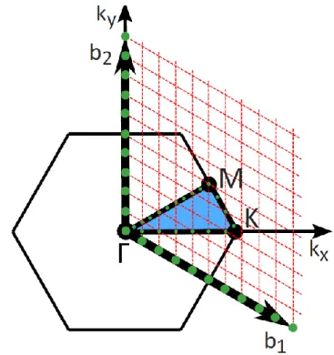
For the orientation of the unit cell we have chosen, namely with 𝒂1 lying on the x axis, they become primitive vectors. The explicit Cartesian form of the allowed k-points on this path is therefore 𝒌𝐾𝑀(𝑖) =2𝜋. 117) Condition (117) means that 𝒌𝐾𝑀(𝑖) lies on the line defined by the section KM moving from M towards K as 𝑖 increases. The final configuration of the group of allowed k-points that we will explore in this work is shown in Figure 15.

Code implementation in Python

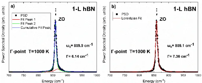
In Figure 18b) we can see the fitting results of the same peak, but with a single Lorentzian function. This claim will be further supported by the temperature dependence of lifetime, which will be presented shortly afterwards. More specifically in the case of phonons, their main interactions occur with other phonons due to the anharmonicity of the interatomic potentials (third and higher order terms in the Taylor expansion).

Results and Discussion

FT k-VACS/Power Spectral Density Spectra

The peaks corresponding to the ZO and the Raman active E2g optical modes are easily identifiable. By simply taking the position of the peak's highest point, we can directly get a rough estimate of the phonon energies. We found this to be true for the vast majority of fitted peaks, therefore the phonon energies can be safely estimated from the position of the center of the peak without the need to perform a fit each time.

Artefacts Induced by the Simulation Parameters

For this reason, we performed experimental runs in which we investigated the effect of time step size, total simulation time, and simulation system size. Therefore, the effect of decreasing the time step size on the spectra is simply to increase the energy range of the spectrum (smaller time steps can detect higher frequency components). Of course, keeping the same time step and reducing the simulation time not only reduces the energy resolution of the PSD spectra, but also results in significantly higher noise.

Phonon polarizations from the cartesian components of the PSD

By identifying the principal component of each peak with respect to the orientation of the k vector, we can identify the polarization of its respective phonon state. An example of the x,y,z-resolved PSD is presented in Figure 24 for a k point along the ΓΚ path at T=300 K for hBN. For this example, remember that due to the particular orientation of the unit cell that we have chosen, all k points along the ΓK path lie on the x-axis.

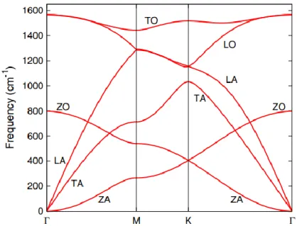
Phonon Dispersion Curves

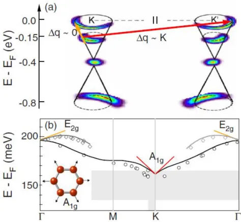
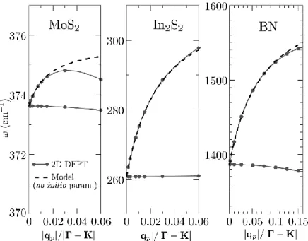
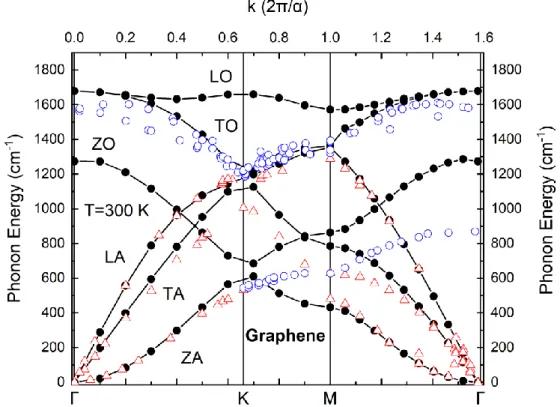
We first note that the behavior of the acoustic modes (hollow triangles) is described with excellent accuracy by our calculations, while the out-of-plane optical branch (ZO) is also described in a very satisfactory way. Also, the description of the LO and TO branches is satisfactory on the ΓM path (parallel to the C-C bond axis), but significantly overestimates about 27% the splitting of the LO branch at the ΓΚ and KM (perpendicular to the bond axis) paths. These results are more or less expected since torsional forces are missing in the framework of the Tersoff potential.

Total and Projected Densities of States

The above observations could indicate that bond bending force constant parameters in the potential are overestimated for monolayer graphene. Nevertheless, despite the potential's lack of complexity, we have seen that it can be satisfactorily used to estimate phonon properties for such exotic systems as monolayer graphene and hBN. On the other hand, for the high-frequency LO and TO branches over the gap, the contribution of the lighter B atoms in the vibrational spectrum is the most dominant, as expected.

Temperature Dependence of Energies and Lifetimes of Zone-Center Phonons

Klemens' model that includes 4-phonon interactions is necessary to properly describe the temperature dependence of the shifts and widths of Raman peaks, Chatzakis et al. On the left we present the decay rate of the SE phonon, while we the right side can see the decay rate of the E2g phonon, along with Time-Resolved Raman. On the left the dependence on the ZO phonon is shown, while on the right we see the dependence on the Raman-active E2g phonon, together with Time-Resolved Raman experimental data at T = 300 K by Katsiaounis et al.