The numbers give the intensities at the corresponding Raman shifts. plus signs) of the olivine Raman spectrum. The numbers give the intensities at the corresponding Raman shifts. plus signs) of the clintonite Raman spectrum. The numbers give the intensities at the corresponding Raman shifts. plus signs) of the lizard Raman spectrum.
The problem of data approximation
Least squares data fitting
Consequently, any multiple of ck can be added to αk without changing the sum of squares of the residuals. Detecting and appropriately handling such dependence and non-uniqueness represents an important task in least squares data fitting. The set of normal equations includes small errors in the coefficients or round-off errors introduced during the solution, which can cause large errors in the solution of the set.
Piecewise monotonic approximation
In Chapter 2, we will see that the piecewise monotone method suggests a completely different approach to smoothing or fitting data.
Non-linear programming problem and Lagrange multipliers
- Non-linear programming problem
- First order conditions for equality constraints
- Quadratic objective function and linear equality constraints
- First order conditions for inequality constraints
The assumption that constraint gradients are linearly independent at the solutionx∗ implies that there exist unique values of the Lagrange multipliers{λi: i=1,2,. We are looking for an estimate of the change {f(x∗+δ)−f(x∗)} caused by the change in the constraints. Although there may be a lot of freedom in δ after the constraints are satisfied, we have the very useful property that the Lagrangian condition (1.18) gives a first-order estimate of the change in the objective function.
M values of Lagrange multipliers are associated with their constraints, one multiplier for each constraint. If the sign is negative, a unit less than bi would decrease the value of the objective function by λi. Minimization of the objective function subject to CTx=ble leads to the same result ˆx, say whether cTi x=bi is present or not.
If x∗ is a local minimum, then it is also a local minimum of the problem of minimizing f(x) subject to the equality conditions. Furthermore, the remarks for the last paragraph of Section 1.2.2 show that if λi is negative, then the objective function can be reduced by changing x∗ by a small amount so that the constraint function ci(x) becomes positive, which preserves feasibility. Ifx∗ is a local solution of the problem that minimizes the objective function (1.14) subject to (1.15), then there exist multipliers{λi:i∈E}, where.
These points correspond to stationary points of the objective function when there are no constraints, because any more away from a Karush-Kuhn-Tucker point that maintains feasibility and that reduces the objective function can only reduce the objective function by ' A quantity that is second order in the change of variables.
The monotonic problem
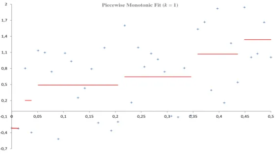
The best monotonic descending approximation is tested as ascending if the order of the data is reversed. We enter the data into L2WPMA with k=1 and obtain the results presented in Table 2.1.
Lagrange multipliers in the monotonic case
We let η be the value that minimizes the expression ∑ti=s(η−φi)2, and by a straightforward calculation we get. As a result, the Lagrange multipliers can be calculated recursively by equation (2.10) in only O(t−s) computing operations as follows. Using the data from the example in Section 2.2, we calculate the Lagrange multipliers and present their values in Table 2.1.
In this chapter we conduct experiments to study how the Lagrange multipliers are changed as the number of monotonic cuts in a piecewise monotonic approximation is changed. To present the behavior of Lagrange multipliers when the number of monotonic parts of the skin increases, we need to define those metrics that present important information about this correlation. For this purpose we will use nine Raman spectrum data files, eight data files of mineral downloaded from Laboratory of Photo-induced Effects Vibrational and X-RAY Spectroscopies, a freely available database on the website [25], of the Department of Physics, University of Parma, and one data file of carbohydrates downloaded from SPECARB, a freely available database on the website [27], of the Department of Food Science, Faculty of Natural Sciences, University of Copenhagen.
A possible relaxation of an inactive constraint reduces the value of the objective function (2.1) by an amount equal to the value of the multiplierλi. It is known that non-zero Lagrange multipliers correspond to active constraints, so a sensitivity analysis concludes that the best fit is strongly dependent on the location of all active constraints. We determine that Y(k,n) is the set of possible vector synRnwithkmonotonic sections that alternately increase and decrease.
SSR=ky−φk2, the sum of the squares of the residuals, the value of the objective function, which is the squared distance between the smoothed values and the values of the function φi, i=1,2,.
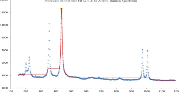
The Raman spectrum of zircon
For k= 3, three monotonic sections, the results of the running program and the calculations are presented in Zircon.xlsx, sheetk=3. As a result, the piecewise monotonic approach in this case detects the main peaks only when ki is even. 16} we will only present figures in which the piecewise monotonic approach detects the main peaks for even monotonic sections.
The piecewise monotonic approximation makes the sum of the squares of the residuals smaller as k increases, preserving the most important turning points. Fork=12 method effectively captures data trends and detects appropriate peaks (see Fig. 3.8). However, we continue to increase the number of monotonic sections, in which the method detects non-significant peaks, to examine the behavior of the measures mentioned in Section 3.1.
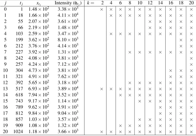
The behavior of the approximation is examined by plotting in Table 3.1 the positions of the turning points by piecewise monotone fits to the zircon data for values of k in {2,4. We notice that the additional turning points of the optimal approximation with k+2 monotonic sections occur between adjacent turning points of the optimal approximation with k monotonic sections. Table 3.2 shows the centralized measurements of the experiment, which are mentioned in section 3.1 for monotonic sections,kin{1,2,.
It is observed that the sum of squares of residuals decreases while the value of the monotonic sections k increases.
Experiments with Raman spectra of minerals
- The Raman spectrum of datolite
- The Raman spectrum of olivenite
- The Raman spectrum of clintonite
- The Raman spectrum of beryl
- The Raman spectrum of lizardite
- The Raman spectrum of hemimorphite
- The Raman spectrum of wulfenite
More specifically, the order of magnitude of the sum of squares of residuals starts from 109forkin{1,2,. The order of magnitude of the maximum absolute value of the Lagrange multipliers decreases from 105forkin{1,2,. In the right part of table 3.5, the positions of the turning points for each fork with optimal fit {2,4,.
It is observed that the values of the sum of squares of the errors decrease as the number of monotonic skin sections increases. The order of magnitude of the absolute maximum value of the fork of the nonzero Lagrange multiplier {1,2,3} is 105. In the right part of table 3.7 we show the positions of the turning points of each optimal fitted fork {2,4,.
As the number of monotonic cuts increases, the order of magnitude of the sum of squares of residuals decreases. In the right-hand side of Table 3.11 we indicate the positions of the turning points of each optimum. As the value of chin increases, the order of magnitude of the sum of squares of residuals gradually decreases.
The right part of Table 3.13 shows the positions of the turning points of each optimally fitted fork {2,4. To investigate the behavior of the approach, we display the turning point positions. In the right part of Table 3.15 we indicate the positions of the turning points of each optimally fitted fork{2,4,.
Experiments on turning point separation
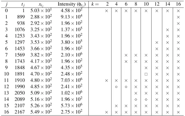
The MS spectrum of diiodothyronine
16}, we obtain the results presented in Diiodothyronine.xlsx, one sheet each for k, with the calculations of the measures under study. In the right part of Table 3.17, we list the positions of the breakpoints of each fork of the optimal fit{2,4,. When k=8, two more turning points occur at positions 2050 and 2087, as indicated by the timestamps in the column marked "8".
So far we have seen that askin increases tok+2 the positions of the pivot points are maintained. It is quite interesting that the fit to this data set shows a shift of some pivot points askin increase by 2. This phenomenon is explained by the property that the optimal pivot point for givenkis is separated by the optimal pivot point whenk+1 (see [15] ).
It is observed that the sum of squares of residuals decreases while the number of monotonic intercepts increases. A reduction in the order of magnitude also occurs in the maximum absolute value of non-zero Lagrange multiplications.
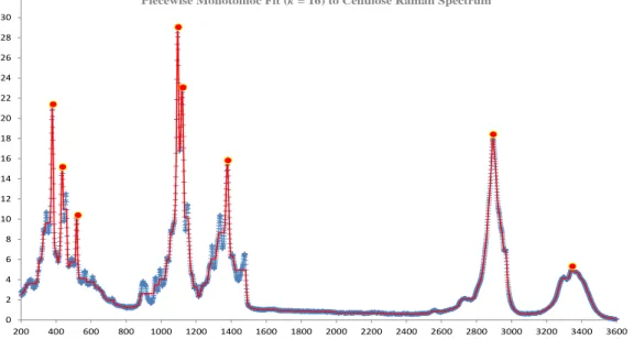
The Raman spectrum of cellulose
While the number of monotonic parts of the skin increases, the order of magnitude of the sum of squares of errors decreases. In this chapter we give the conclusions about the experiments, mentioned in chapter 3, which can lead to the determination of the relationship between the number of monotonic cuts and Lagrange multipliers in a piecewise monotonic approach. Next, in chapter 3, figures and tables with the results of the calculations were presented to capture the main characteristics of each data set.
The maximum absolute value of estimated errors also decreases as the number of monotonic sections increases. Moreover, the order of magnitude of the maximum absolute value of nonzero Lagrange multipliers increases as the number of monotonic sections increases and the method detects not so important peaks. As comes from the theory of general nonlinear programming, the magnitude of the Lagrange multipliers gives an indication of the importance of the corresponding constraints, and also shows the magnitude of the change of the objective function with increases.
This will be very valuable for the development of a Lagrange multiplication test that will provide an estimate of an appropriate or sufficient number of monotonic sections of the fit. Gauss, Theory of the Combination of Observations Least Subject to Error, Part One, Part Two, Supplement, Classics in Applied Mathematics, Society for Industrial and Applied Mathematics, facsimile edition, 1987. Lu, “Signal Restoration with Controlled Piecewise monotonicity reduction”, Proceedings of the IEEE International Conference on Acoustics, Speech and Signal Processing, May 12, 1998 - May 15, 1998, Scattle WA, vol.
Yuan, A review of subspace methods for nonlinear optimization, Proceedings of the International Congress of Mathematics, pp.