If the predictions are inaccurate, the performance of our algorithm falls back to that of the optimal online algorithm. In these problems, the predictor can predict the states of the optimal algorithm at each time step.
Contribution
If the optimal algorithm makes decisions based on the entire input, the oracle predicts the states of the optimal algorithm. The error is defined as η=S−OP T, where S is the cost of the predicted solution and OPT is the cost of the optimal solution. The error is defined as the ratio ℓ1 between the true and predicted edge death times.
Organization
In this way, we have embedded the intricacies of the optimal algorithm in the predictor. This algorithm will be extended to be used in the online instance of the problem. In the case of uniform cost, it is assumed to be a constant approximation of the optimal algorithm (see Appendix B in [35]).
Online Algorithms
Competitive Analysis
We denote by OP T the optimal offline algorithm for the problem P and by OP T(σ) the cost of the solution generated by OP T on the input sequence σ ∈ I. Competitive relation) We say that the online algorithm ALG for the minimization problem P is c -competitive, if for each input σ there exists a constant a >0 such that. On the other hand, the objective of the adversary is to create the worst possible sequence of requests for the online player and at the same time the best sequence for the optimal offline algorithm. In deterministic algorithms, the adversary knows in advance how the web algorithm will respond to each request.
Paging
- Deterministic paging algorithms
- Randomized paging algorithms
The competitive ratio of any online random algorithm for the page problem is at least Hk, where Hk is the k-th harmonic number. We now define the M ARKER algorithm, which is a modification of the M ARKIN G algorithm we presented in the previous section.
Metrical Task Systems
Combining online algorithms
However, the competitive ratio c of a learning-enhanced algorithm is a function of the predictor h and the error and therefore we write c=c(h, η). Furthermore, we will normalize the error η with the cost of the offline algorithm OF F, as we discussed in the previous chapter. Replacing N −r with k in the results of the previous section yields the optimal bounds proven in [66].
Basics of Learning-augmented Analysis
Ski rental
- The problem
- Ski rental with predictions
- Robustness-consistency trade-off
In the online setting, the skier does not know in advance the number of skiing days T. The essence of the problem lies in the skier's uncertainty about the future. If the oracle predicts that the skier will ski for more than b days, Algorithm 1 buys the skis a little earlier than A.
Non-clairvoyant job scheduling
- The problem
- Non-clairvoyant job scheduling with predictions
- Robustness-consistency trade-off
An important aspect of Algorithm 5 is that it implies a trade-off between robustness and consistency. As in Ski Rentals, we observe that there is a trade-off between robustness and consistency. We note that in the case of n = 2 there exists a better algorithm that achieves the optimal trade-off.
Designing learning-augmented algorithms
In the online version of the problem, the elements of U are revealed in an online way. Algorithm G is known to be an O(logT) approximation of the optimal algorithm, even in the case of non-uniform acquisition costs. Finally, an important result would be to prove that algorithm G is a constant approximation of the optimal algorithm in the case of uniform cost.
Paging with predictions
Paging with predictions
- Marking algorithms
If the predictions are accurate, the error will also remain constant, but the normalized error will be smaller since the length of the sequence will be larger. When all the elements of the cache are marked and a cache miss occurs, a phase ends and we unmark all elements. The following two theorems relating the performance of the optimal and marker algorithm to the number of clean elements hold [31].
Predictive Marker
We could increase the length of the sequence without changing the value of the optimal solution or the impact of the prediction. If the predictions turn out to be inaccurate, we'll switch to a classic tagging algorithm that will uniformly and randomly weed out untagged elements. The total length of the chains is equal to the total number of cache misses caused by our algorithm.
BlindOracle
- Combining online paging algorithms
- Analysis of BlindOracle
Let ∆P and ∆D be the changes in primary and dual costs, respectively, in a particular iteration of the algorithm. We will now present an application of the learning-augmented primal-dual method to the parking permit problem [54]. The configurations (basics) and costs of both algorithms are the same up to time step t-1.
Metrical Task Systems with predictions
Follow the Prediction
We will now formally define the Follow the Prediction (FtP) algorithm and analyze its performance. We define Follow the Prediction (FtP) as follows: at time t, after receiving task ℓt and prediction pt, FtP goes to state. Algorithm F tP achieves a competitive ratio of 1 + OF Fη , where η is the prediction error with respect to OFF.
Caching
In the online environment, the limitations of the primordial program are given one by one as new elements are revealed. The error can be defined as the cost of Shortest Predicted Job First (SPJF) algorithm minus the cost of the optimal algorithm. The next crucial idea was the trick with the (meta-)algorithm At, which was also used in the analysis of the learning augmented algorithms for the MTS problem in the previous chapter.
The Primal-Dual method with predictions
The primal-dual method
First, we are going to demonstrate the primal dual method in the standard case of online algorithms without predictions. Moreover, the algorithm can increase the value of yj only in the round it is first given. Proof of (2): When the algorithm updates the primal and dual solutions, the change in the dual gain is 1.
Learning-augmented primal-dual method
Next, notice that the algorithm never updates any variablex≥1, since it cannot be in an unsatisfied constraint. The proof of this theorem is very similar to the proof for the classical online algorithm. To prove consistency, we split the primary growth into ∆Pc which indicates the primary growth due to aggressively updated groups (i.e. groups in predicted solution A) and ∆Pu for groups not in predicted solution.
Applications
- The Parking permit problem
- Extensions to leasing problems on graphs
Suppose we have two bases with the same expected elements for k elements, 0≤k≤r, where r is the rank of the matroid. We denote by OPT1 and OPT2 the execution of the optimal algorithm in the two instances respectively. We know of no uniform cost example where G is not a constant approximation of the optimal algorithm.
Job-Scheduling revisited
Prediction error
For each instance of the fuzzy scheduling problem with predictions, the prediction error is defined as Clearly, this error is neither monotonic nor Lipschitz, since SPJF produces an optimal solution if and only if the order of the predicted jobs is correct. Finally, we note that the error measure must account for job identities, since the cost of the optimal algorithm will be the same for every permutation of the actual job sizes, but the error will change.
Job-scheduling with predictions
However, real-world problems require one to solve an instance of the same problem repeatedly. For the following, we assume that all elements of the matroid have unit costs and that at most one edge dies at each time step. Suppose we have an example of the MMM problem for uniform matroids with N elements/pages that live at each time step (see the online approach in section 2) and that at most one element dies at each time step.
Changing Bases with predictions
Preliminaries
- Matroids
A maximally independent set—that is, an independent set that becomes dependent upon the addition of some element of E—is called a basis for the matroid. A circuit in a matroid M is a minimal dependent subset of E—that is, a dependent set whose proper subsets are all independent. We define the rank of an arbitrary set S to be the cardinality of the maximal cardinality independent subset of S.
Multistage Matroid Maintenance (MMM)
- The problem
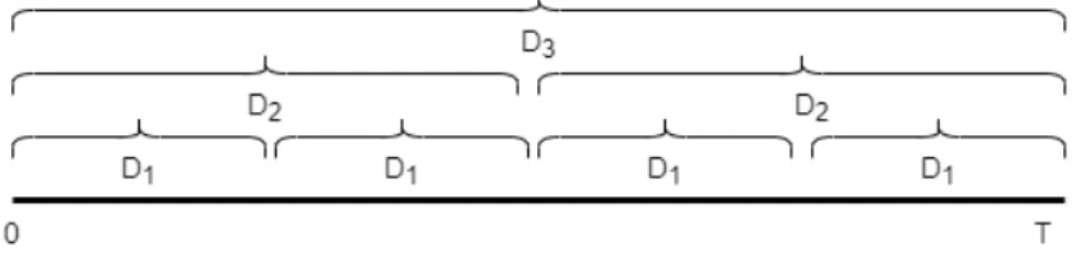
- The interval model
- Offline MMM
- Online MMM
- MMM with uniform costs
- The greedy algorithm
In [35] they give an LP rounding algorithm that is an O(logrT) approximation in the general case and an O(logr) approximation in the uniform cost case. Note that the greedy algorithm is not optimal even in the case of graph matroids. It is easy to extend Algorithm G in the case where multiple elements can die at each time step.
Combining online algorithms
That is, we buy the edge that dies furthest into the future, so our set remains independent.
The learning-augmented setting
Analysis of B
For uniform matroids, a better dependence on η is possible, as we will prove in the next section. Combining Algorithm B with Online Algorithm A using the results we presented in Section 3 yields the following theorem.
Uniform matroids
Caching
The element we evict from the cache, to make room for the input element, is moved to the base array S′. From the MMM perspective, the optimal algorithm is to buy the element that dies furthest into the future. This theorem also implies a lower bound for the case of uniform matroids that we considered in the previous section.
Generalization
On the other hand, from the perspective of the MMM problem, an element is dead and we need to buy a new element to form a base. In fact, the true dead time ti of elementei must be less than all the respective times of the newly added elements of G. Thus, elementei forms an inversion with at least one of the newly added elements of G.
Conclusions
We claim that one newly added element of G in the cycle forms an inversion with element ei. Furthermore, the predicted death time t′i of ei must be greater than that of the newly added elements otherwise algorithm B would have chosen one of these elements. Finally, we note that in the case of elements with non-uniform acquisition costs it has been proven that our predictions cannot help us go beyond the classical online algorithms, even in the case of uniform matroids [9].