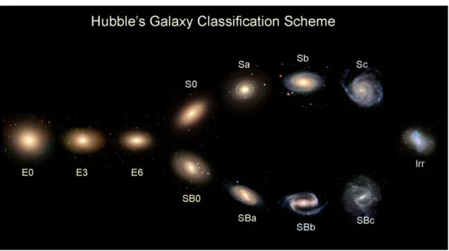
Hubble began a systematic research and he not only classified galaxies into types in the so-called "Hubble's Tunning Fork" diagram (see figure 2.2), but he also discovered the expansion of the universe. The first one, the CfA (Centre for Astrophysics), provided a first discrete implication of the large-scale structure of the universe. The fuzzy picture of the structure of the universe became clearer as more redshift surveys followed.
The disk contains mostly younger stars, gas and dust, and the arms of spiral galaxies are located here.
Clusters and Groups of Galaxies
The fraction of Spirals and Irregulars decreases dramatically as the density increases, while conversely the fraction of ellipticals and SOs increases in high-density regions (Dressler et al. 1997). Recent studies (Poggianti et al. 2009, Xin-Fa Deng et al. 2009) confirm this result and raise an interesting question whether this dependence is a result of the initial galaxy formation process or an evolutionary effect. Irregular clusters: They consist of 40% spiral galaxies and they have a lower velocity dispersion than ordinary ones.
They appear fainter than usual in x-rays and appear to include galactic substructures.
Superclusters: Clusters of Clusters
Other components of the cosmic foam are the sheets or walls which, as their name suggests, are thin (2D) formations. In figure 2.8, the large scale of the universe as constructed by the 2dF Galaxy survey can be seen. Some specific structures such as the aforementioned Sloan Great Wall and the Shapley Spercluster can be distinguished.
Voids
Some specific structures such as the named Sloan Great Wall and the Shapley Spercluster can be distinguished. produced 3-D cosmic maps that established void space as the dominant component of the Cosmos, occupying about 95% of its total volume. The inner empty regions expand outwards with greater acceleration than the outer ones, and during the decisive process of shell crossing, the former pass over the latter, so that the mass distribution of the interior is evened out, and voids are gradually led into expansion and increasing "emptiness00. The various accumulation of the inner and outer shell of the cavity also results in the formation of ridges against the edges of the cavities.
During the last decades, voids have been a field of great research interest because, apart from being crucial for the understanding of the structure and dynamics of the cosmos, they can shed light on the underlying cosmological scenario and on cosmological parameters.
Studying Matter Distribution
Cluster Analysis and Percolation
- Percolation
- Applications of percolation
- Cluster Analysis
- Types of Clusters
- Applications of Cluster Analysis
- Cluster Analysis and percolation used in Cosmology
The behavior of different percolation models is likely to be described by some universal parameters in the vicinity of the critical probability pc. These characteristics of a percolation transition are expected to depend only on the spatial dimension of the system and the percolation model. They are independent of microscopic details such as lattice structure or whether percolation is considered to be bond or site.
In the case of the percolation problem, the proportion of occupied sites in the clamped cluster plays the role of an order parameter. By convention, the percolating clusters, or in other words the clusters connecting the lattice boundaries, are not included in the calculation of the quantities ns(p), ws(p), S(p). However, in the limit of infinite lattice size, the average cluster size appears to be a single one near the percolation critical point.
The term does not refer to a particular algorithm or method, but to the task itself, which is to find an underlying context or structure of the data. However, the definition of a cluster is imprecise and the best definition depends on the nature of the data and the desired results. Meaningful clusters are called classes, and they are supposed to capture the natural structure of the data.
Each cluster node of the tree is the union of its subclusters children and thus objects belonging to a child cluster also belong to the parent cluster. By choosing a level of the dendrogram and cutting it off one can obtain partition clusters (see Figure 2.13). Cluster analysis has been applied to find patterns in the atmospheric pressure of polar regions and parts of the ocean that significantly influence continental climate.
But later it was proved that this scenario does not reproduce the structures of the observed universe.
FOF Method
The Main Code
Statistics Application
In order to define the clustering provided by our percolation algorithm and also to use statistics, it is essential to develop an additional piece of code that will compute some statistical properties of the clustering system. Properties of the largest cluster, the largest cluster is defined as the one with the largest mass number, i.e. the largest number of cluster members, the diameter of the largest cluster (the code calculates the distance between all cluster members and identifies the largest clusters). of all distances as the diameter of the largest cluster) and the mean diameter of the largest cluster (which is defined as the mean of all distances calculated between pairs of members of the largest cluster: Dmean=Σrpair/N.). In other words, the number of points in the distribution found in clusters for a given value of the percolation radius Rp relative to the total number of points.
For example, in a distribution, for a particular Rp, the code calculates that there are 3 clusters of set 2, 4 clusters of set 5, and 2 clusters of set 10, etc. is. In the next chapter, we also apply this statistic to random samples of the same number of points as data distributions, produced using a random number generator, to compare the random sample's behavior with that of N-body simulation samples from the same population .
Need for Repetitions: The code’s main caveat
Now, after checking, the code correctly assigned pair (7,8) to the same group as (4,7), but d(2,7) did not change and thus a point was incorrectly assigned. Instead of tracking group "1" including members 2,4,7 and 8, the code incorrectly tracked two clusters: group "1", including points 4,7 and 8, and group "2", including points 2 and 7. We explored different ways to develop the code using single vectors instead of duals, which could alleviate several problems we encountered and speed up the algorithm.
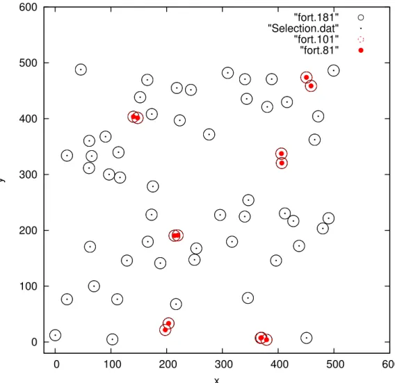
Example: Application on a 2D-distribution
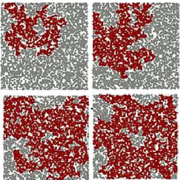
Small clusters merge to form larger ones and the system tends to form a large cluster that will contain all the points or in other words the system tends to penetrate. For Rp = 55 the system is not yet penetrated, but almost all points belong to a single cluster.
Numerical Data
Code application and performance of different statisticsstatistics
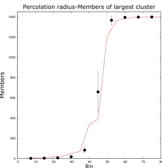
- Members of largest cluster
- Mean Diameter of largest Cluster
- Diameter of largest Cluster
- Fraction of percolated halos
- Multiplicity Function
The spread is reached at Rp = 65M pc for subsample A and Rp ∼62M pc for the random distribution. In this and the following diagrams 4.2–4.8 the red line corresponds to the results for simulations of dark matter haloes and the black dots with error bars represent the results for random distributions. We see that for Rp < 40−45M pc the halo structures are significantly larger than those of the random data, indicating strontium accretion of massive dark matter haloes.
As in 4.3, we see that for Rp <40−45M pc the largest cluster of the distribution is significantly larger than the random data, indicating the strong clustering of massive dark matter haloes. As in Figure 4.4, we see that for Rp <20−25M pc the largest cluster of the distribution is significantly larger than the corresponding random one, indicating a weaker cluster of dark matter haloes compared to the more massive halo sample shown in Figure 4.5. Figures 4.7 and 4.8 show diagrams of percolation radius - Fraction of percolated points for both subsamples A and B and random distributions of equal numbers.
For different values of radiusRp, we examined for the subsamples, A and B, the frequency of occurrence of the multiplicities of different clusters and also of the corresponding ones from the random simulations. For the random data, we found the mean frequency and standard deviation as obtained from 100 simulations of 1399 objects and . In all the multiplicity function diagrams (Figures 4.9-4.12) we can see that for small numbers the frequency is lower for the dark matter halo samples than for the random ones.
As the abundance increases to intermediate values, the frequency is nearly the same for both N -body and random simulations, and for even larger abundances, the frequency is significantly larger for the N -body simulation subsamples than that observed for the random simulations. The comparison of the behavior of random and N-body simulation systems indicates that the latter are significantly more clustered as they form larger structures for the same value of percolation radii.
Conclusions
This behavior is seen in all four multiplicity function diagrams, but it is more apparent for diagrams 4.10 and 4.12, which correspond to larger Rp values than 4.9 and 4.11, respectively, and thus many more multiplicities are observed. Also, both halo subsamples form larger percolating structures than their respective random distributions up to a percolation radius of Rp = 40−45 Mpc for subsample A and Rp = 20−25 Mpc for subsample B, indicating strong clustering in the gravity systems of N bodies. Similarly, in Figures 4.7 and 4.8 we can see that the fraction of haloes in clusters with respect to the total number of haloes is significantly larger for the N-body samples up to the same values of percolation radii Rp as before.
We also observe that the clustering is much stronger for the more massive dark matter halo of sample A with respect to sample B. In addition, we have presented characteristic multiplicity function diagrams for both subsamples, A and B, and also for the corresponding random simulations (Fig 4.9-4.12). In all four diagrams, random simulations form more low-multiplicity clusters than the dark matter halo samples, while the frequency of higher-multiplicity clusters is greater for the dark matter halo samples than for the random simulations.
It is also interesting to note that in some cases the largest multiple structures in the halo distributions are not reproduced at all in the random samples. This clearly shows that the randomly distributed blobs are more evenly distributed and much less clustered on large scales than the gravitationally interacting haloes of the N-body simulation. To summarize, the entire statistical test performed on clusters penetrated haloes and the corresponding random distributions clearly indicate the existence of significant gravitational clustering, significant in the flat ΛCDM cosmological model.