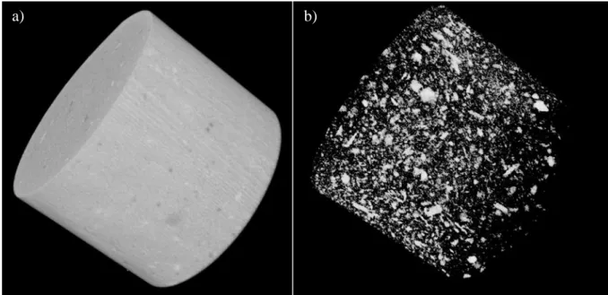
1.4 : Representative illustration of the phenomena that take place at the interface between calcium phosphate cement and the surrounding environment during hydrolysis: (1) dissolution of biocement; (2) precipitation from solution; (3) ion exchange and structural rearrangement and crystal growth (17). 3.2 : Typical SEM image of granules collected from the α-TCP powder used for this work (51).
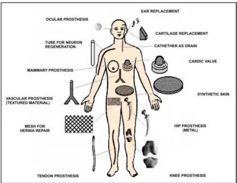
Information about biomaterials and bone cements
Recrystallization can occur in parallel with the change in crystal size and phase transformation (12). Last but not least, there is little information in the literature on the stresses induced during the fabrication of self-hardening cement.
Thesis goals and structure
As demonstrated in Chapter 2, most studies dealing with CPCs measure their strength by performing compression tests only. Moving on to Chapter 5, the experimental results of the developed strains, obtained through three characteristic stages during the material preparation, are presented and discussed: (i) solidification (ii) curing and (iii) re-immersion.

The solid foams obtained were shown that the addition of gelatin improved the cohesion and injectability of the cement paste. This makes it unclear whether various properties, including mechanical ones, of the extruded cement are still clinically acceptable (40).
Materials used and sample handling
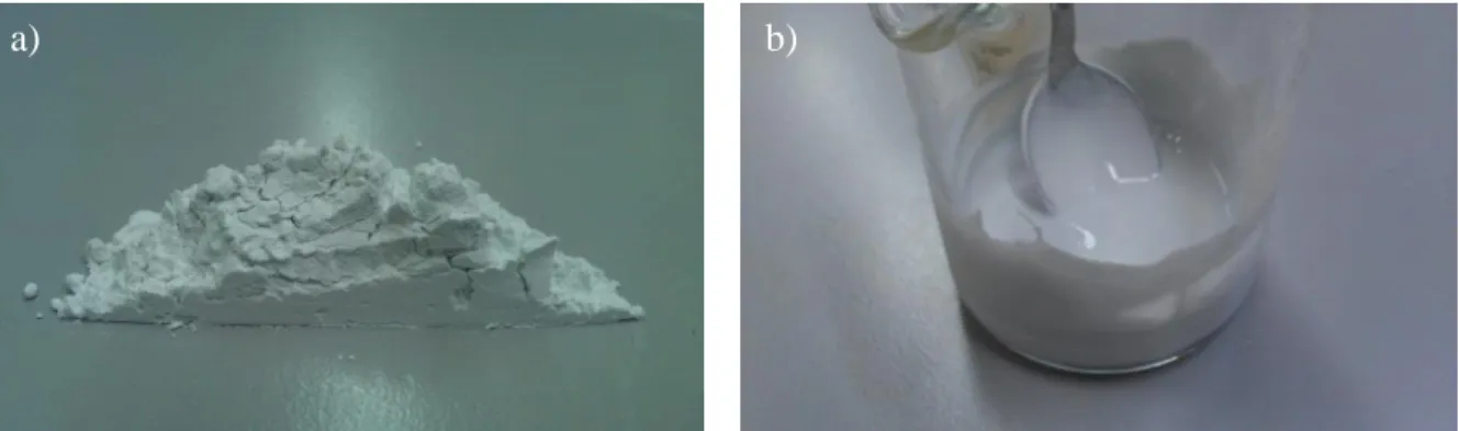
The fabrication of the samples was carried out through three different steps and more specifically: (I) manual mixing of α-TCP powder and Na2HPO4 aqueous solution, in a ratio of 1 ml : ~ 2.06 gr, which resulted in a malleable paste (Fig. . 3.1b) and poured with a spatula into molds (II), the poured paste is allowed to harden for at least 4 days, at room temperature (~23 0C) and (III) the hardened samples were recovered and placed in Ringer . solution that has acted as a fortifying fluid, as reported in the literature (27), for at least 15 days. The hardening process also took place at a temperature of ~23 0C except for a number of specimens intended for low load insertion (see 4.3.2.2), which were hardened at human body temperature (~37 0C).
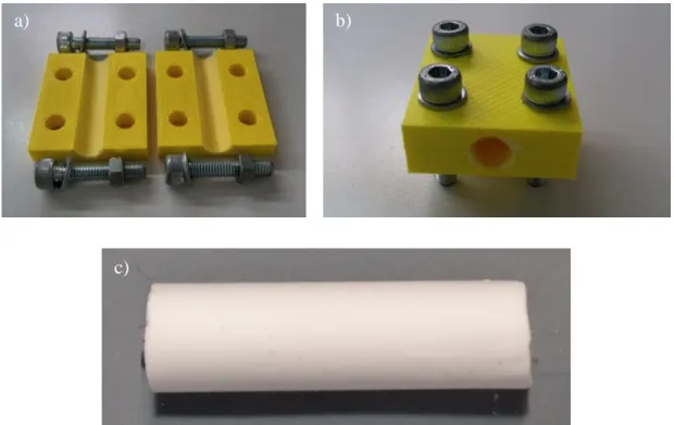
Moulds design and samples geometry
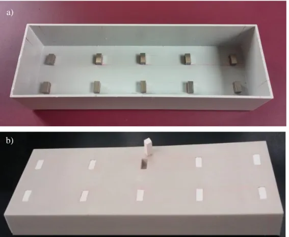
As a result, two new cylindrical specimens of 12 mm in diameter and 20 mm in length were created and designated as AW1 and AW2. The third mold (Type III) was made of aluminum with a cylindrical cavity 12 mm in diameter and 40 mm in length.
Microstructural changes
- Scanning Electron Microscopy
- X-Ray Diffractometry
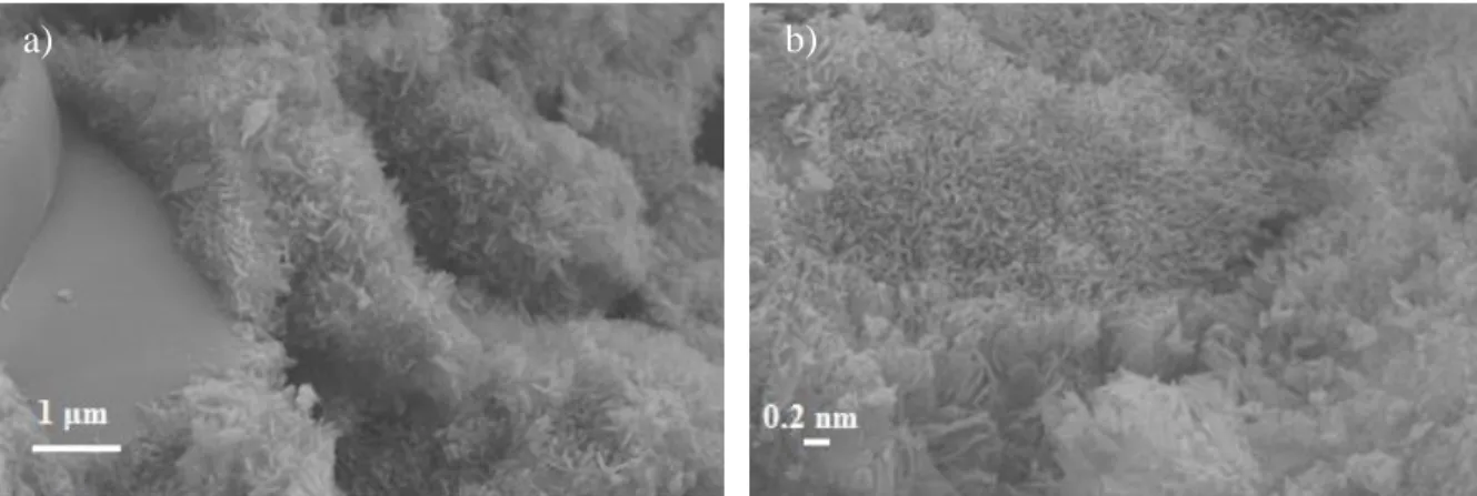
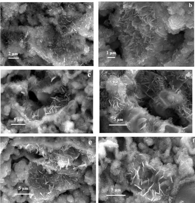
In the following days, the entanglement became more complex, as shown in the captured images after 8 and 10 days (192 and 240 hours) of immersion. Finally, residual α-TCP was detected for the last time in the samples recovered after 7 days of immersion in the curing liquid.
Porosity investigation
- Micro computed tomography imaging
- Microscope investigation
- Confocal microscopy
Thus, the distribution of crystals has a significant influence on the mechanical behavior of the material. Characteristic images were captured and then processed with software to estimate porosity based on occupied pore surface area.
Mechanical properties
- Compressive testing
- Low-load indentation
- Room temperature
- Body temperature
- Diametral Compression Test
- Failure model
Where (P) is the applied load and (S) is the stiffness (𝑑𝑃 . 𝑑ℎ), in the unloading section, which was calculated by linear fitting of the first 25% of the unloading curve. As can be concluded, the obtained Young's modulus of the studied material after curing in Ringer's solution for 14 days based on pressure tests (4.3.1) is significantly higher. The reason is to investigate any changes in the final mechanical properties of the CPC under investigation due to increased temperature during the curing period.
Therefore, entanglement of precipitated CDHA crystals appears earlier than in CPCs solidified at room temperature. 4.18 : Representative load-displacement curves of diametral compression tests on dry and wet CPC specimens.

Absorption phenomenon
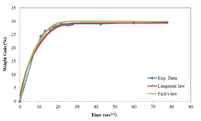
Each time the sample was recovered from the liquid medium and before weighing, it was gently shaken to remove the excess liquid on the surface of the sample. As is evident, the weight gain develops rapidly during the first three minutes, while after 14 minutes more than 85% of the total absorbed liquid medium has been achieved. Therefore, the time period of the first 15 minutes is the most decisive for the absorption phenomenon.
To ensure that the results were unaffected by the geometry and size of the sample, the experiment was performed again using a small block sample (dimensions: 6x6x12 mm). It is clear that they are practically the same when compared to the results obtained from the cylindrical sample, except for the first two minutes of immersion.

Implemented method
- FBG working principle
- Isostrains justification
- Multiplexed sensing
Therefore, the stress field in the center of the specimen, where all FBG sensors are placed in this study, is certainly not affected by edge effects. In addition, when the cylindrical sample is subjected to an external stress, a fraction of the applied stress is transferred to the embedded FBG. The degree of strain measured by the FBG is highly dependent on the ratio of the volume stiffness between the host material and the fiber (82).
Therefore, these values of the stiffness ratio are of significant magnitude and it is therefore possible to consider that the isostrain assumption is satisfied and the measured strains on the FBG sensor can be considered equal to the axial strains on the host material (83). As a result in this work, apart from using single FBGs, serial multiplexing also helped the study of the strain field of the host material to interrogate a wider area as well as to confirm the results obtained from.

Experiments
- Technical details
- Single FBGs
- Multiplexed FBGs
- Results
- Solidification
- Hardening
- Re-immersion
As a result, any slight variation in these parameters could have resulted in differences in the size of the strains obtained. As can be observed the values of the displayed stresses, when the specimens were first immersed in the curing liquid (0 days), are between -420 με and -183 με, which is comparable to the range of the exposed strain obtained by single FBG (~-390 με and ~-244 με). The low magnitude of the strains obtained, also confirmed by the multiple FBGs, suggests that no significant residual strains were generated during immersion of the bone cement in Ringer's solution and subsequent hardening.
More measurements were also taken from the Bragg sensor in the following days, every 24 hours, until saturation levels were reached and the calculated strains are shown in Fig. It is noted that the changes in the recorded strain values can be attributed to the fatigue of the interface between the FBG sensor and the bone cement material, due to the successive drying-swelling process it has.

Introduction
In the case of the finite element method, the surface or volume to be modeled is divided into smaller, elementary parts (Fig. 6.2). A number of parameters affect the accuracy of the results obtained from a finite element analysis (FEA). For example, the error of the results depends on the size of the elements, in relation to the dimensions of the modeled area, especially in regions where the investigated fields can vary with high gradients, or complex phenomena are simulated, e.g.
Furthermore, the accuracy of the results obtained from an FE Analysis is related to the distortion to which the elements are "subjected" to the analysis, especially in the case of a 3-D model. In general, no simple rule applies to the number, size, and geometry of elements to be used in a developed model, and only a posteriori parametric study can provide information on the reliability of the results (85).

Absorption phenomenon and developed hygro strains
Since the weight gain results, in each time interval, were considered to be the sum of the calculated (𝑢) values of all calculated time intervals. Subsequently, a simulation model was developed in the Abaqus® simulation software package for the calculation of the induced hygro-tensions due to the absorption phenomenon. The optical sensor was also simulated, which was located in the longitudinal axis of the specimen.
Several runs were performed giving different values to 𝛽𝑠𝑖𝑚 in order to optimally fit the simulation results with the experimental data (hygro strains) obtained from the first run of the corresponding experiment (see section 4.4). Although the 𝛽𝑠𝑖𝑚 obtained from the simulations is similar to that calculated from the experimental data in section βI=7.02x10⁻⁶/%w/w), this modeling of the diffusion phenomenon and induced hygrostam presented above is considered a simplified approximation of the corresponding phenomena for two main reasons.
A case study of CPC medical application: Total Hip Replacement
- Where Total Hip Replacement is implemented?
- Modeling
- Results
6.10: A human femur consisting of the trabecular bone on the inside and the cortical bone on the outside (96). Based on the CAD model of the stem implant, a new structure was created that surrounded the stem implant and simulated the bone cement. As can be seen in the bottom of the cavity, on which the lower part of the stem rests, the stress values have the same high value (45 MPa).
6.18 : A free body cut (dotted line) in the center of the specimen, perpendicular to the longitudinal axis, and its projection on the cut plane to the inside of the bone cement. The same loading scenario was run again, but this time the Young's modulus of the bone cement was set to 1.7 GPa.

Conclusions
It is noted that the method applied to investigate crystal distribution (μ-CT imaging) may also be useful in studies where crystal distribution is modified by the addition of additives to the calcium phosphate powder. The porosity of the material also includes the cavities created due to the entrapment of air during the pouring of the paste into the molds. The volume of adsorbed liquid coincides with the total pore volume of the material, suggesting the following: (a) an interconnection of the pores (b) in this time period diffusion can be considered negligible.
From the obtained results of a static analysis run, it can be concluded that the highest stress values in femur bone and stem implant structures are displayed in the anterior and posterior side of the same longitudinal area (middle of femur bones' upper part). In bone cement structure, the highest stress values are displayed in the bottom of the cavity, where the lower part of the stem rests.
Future work
Calcium phosphate ceramic systems in growth factor and drug delivery for bone tissue engineering: a review. Effects of hydroxypropyl methylcellulose and other gelling agents on the handling properties of calcium phosphate cement. Effect of different cellulose ethers on both handling and mechanical properties of calcium phosphate cements for bone replacement.
Influence of anti-leaching agents on the rheological properties and injectability of a calcium phosphate cement. Monitoring of hardening and hygroscopic induced strains in a calcium phosphate bone cement using FBG sensor.