Physical Activity Prediction Using Machine Learning on Wearable and Mobile Devices

One of the most important aspects in such approaches is the algorithm used in the goal-setting process, as appropriate goal-setting methodology has been shown to actually lead to an increase in PA levels. We exploit the publicly available datasets related to the COVID-19 pandemic [12] to establish the correlation between the COVID-19 movement-restrictive policies and the predictive ability of ML models used to predict a user's daily step count.

Figure 1.1: Applications of step count tracking in various devices

Wearable Devices and Adaptive Goal Setting

This research showed that the personalized approach outperforms fixed goal setting in increasing an individual's PA levels. The relevant literature using adaptive goal setting is presented in more detail in Chapter 3.

Figure 2.1: Fitness tracker market by device type [54]

ML and Time-Series Analysis

In Table 2.1 below we summarize the characteristics of the different goal setting methodologies. In this work, we will focus on supervised ML techniques to perform a continuous analysis of time series PA data and design a model capable of predicting the daily PA of a user in the form of the number of steps taken during a day.

Figure 2.4: ML categories and applications [26]

Goal Setting Approaches & PA

In [63], the impact of context-aware personal goal setting was evaluated through tests on a context-aware and an active control group. Finally, in [48], an idiographic (person-specific) approach has been tested to establish the effectiveness of dynamic models of PA in the context of goal setting and positive reinforcement interventions.

Context-Aware Coaching & PA

Once again, the results indicate that personal goal setting is more effective in increasing PA levels as expressed through the daily step count. Our work is relevant to the above studies as it uses a variety of contextual and personal features to effectively predict a user's daily step count.

ML Prediction models & PA

In [38], the authors developed a neural network model that took into account a number of contextual characteristics derived from questionnaires (personal, social and environmental characteristics) as well as daily step counts over a period of one week (7 days) and predicted the average weekly number of steps individual. In our work, we also use contextual and personal characteristics, but regardless of the research described above, we train the model over a period of 5 days to obtain a prediction of the estimated number of steps for the next day (day number 6).

Intervention Through Wearable Devices

Related Work Limitations

Our work differs as it provides evidence (through evaluation) about the effectiveness of the recommended algorithm. First, while in [38] 3 different activity tracking devices (FitBit Charge, FitBit One and FitBit Zip) were used, they are all different models of the same brand and no integration framework is mentioned in the research. Next, in 4.5 we examine the necessity of reducing the number of features in the original data set.

In this section we present the two different approaches tested to reduce the dimensionality of the original.

Table 3.1: Example of how MAE is not indicative of a regression’s algorithm efficiency

Data Collection

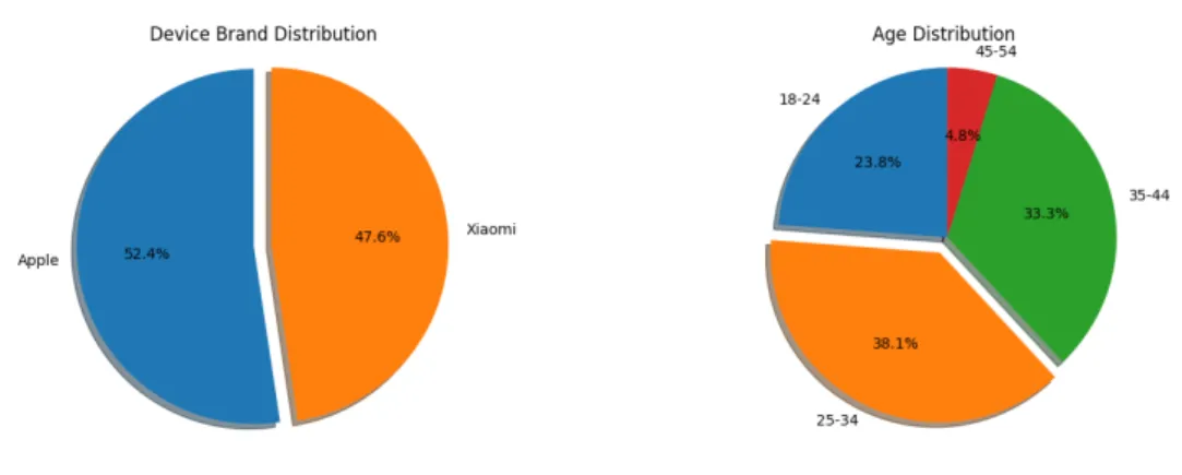
As mentioned above, all participants were users of either an Apple or a Xiaomi activity tracking device. Since all the participants' native language is Greek, the language used in the questionnaires was also Greek. For two of the questionnaires originally published in English, a formally published Greek translation was used.

We also described the sample population that was considered in the data collection process, with the nature of the data collected.

Figure 4.2: Device type and age group distributions in dataset

Data Preprocessing

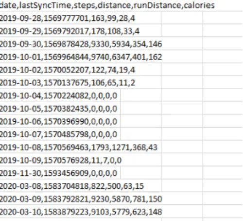
The format of the Apple data after the time-related preprocessing was as in Figure 4.7 below. After applying the integration process described in 4.2.1, the format of the activity data recorded from the different activity tracking devices was as shown in Table 4.1. The sub-datasets were written to separate files to be parsed later in the next stages of the transformation process.

To clarify this statement, a blueprint of the data sets taken after this process is presented in table 4.8.

Figure 4.5: Apple & Xiaomi raw activity data

Initial Feature Selection

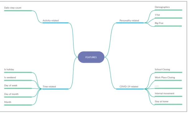
Our approach to this initial feature selection process (feature selection is also done in part . "model development" of our methodology 4.5) was to determine the value of each of the 4 categories by training ML models with different subsets of features. 4 ML regression algorithms were fitted to each data set and the best performing models were compared to decide whether the contribution of each set of features has a positive impact on the efficiency of the predictive models. In this section we have described the last stage of the part of our methodology that deals with the creation of the data set.

We described the approach taken to select the feature categories to be included in the final dataset and also presented the experimental process, which proved that our C2 contribution was valid, as all feature categories were found to contribute positively to the predictive ability of the ML models.

Figure 4.9: Schematic representation of the different feature categories

ML Algorithm Selection & Optimization

In the next section, we present the first phase of the model development process, the process of selecting the best performing ML regression algorithm and optimizing its performance through hyperparameter tuning. In the next subsection, we present the approach used to define the optimal configuration of the prediction algorithms. This is an essential step to obtain the best possible performance of the forecasting models.

By applying this method to all tested ML algorithms, we obtained the best performing hyperparameter configuration for each model.

Dimensionality Reduction

Based on the above, it was decided that it would be appropriate to test whether reducing the number of features would lead to an improvement in the performance of the developed ML models. In order to reduce the dimensions of the data set, 2 different categories of such testing methodologies, feature selection and dimensionality reduction by projecting the data set into lower dimensions, were selected. The results of the PCA approach adopted to reduce the dimensionality of our data set can be found in 5.4.2.

In this part of our methodology chapter, we discussed the different approaches tested in reducing the dimensionality of the original data set used in our experiments.

Figure 4.10: Pseudo-code for the Recursive Feature Elimination (RFE) algorithm [11]

Obtaining Optimal Window Size

All approaches and techniques presented in Chapter 4 are evaluated using the evaluation methodology described in 5.1, and the results of this experimental process are presented together. Multiple regression algorithms were used throughout this process and many different approaches were used at different stages of the research. Later, in Section 5.4, we quote the results of two different approaches implemented to reduce the number of features in the data set, RFE and PCA.

In the next section, Section 5.5, the results of the experimental process of identifying the optimal number of days to use as input are presented.

Figure 4.11: Number of dimensions and available data in dataset, in relation with the window size n

Evaluation

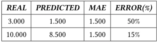
Even those that report adequate performance [38] do not report MAPE or any other similar metric or even the range of daily step counts in the dataset to gain more insight into the predictive abilities of their models. First, the performance of the model was evaluated using the CV procedure on the training data. The CV procedure considered both metrics discussed in 5.1.1 to evaluate the performance of the algorithm.

The values of the MAE and MAPE metrics were calculated from the model predictions, completing the evaluation process.

Selection of Important Feature-groups

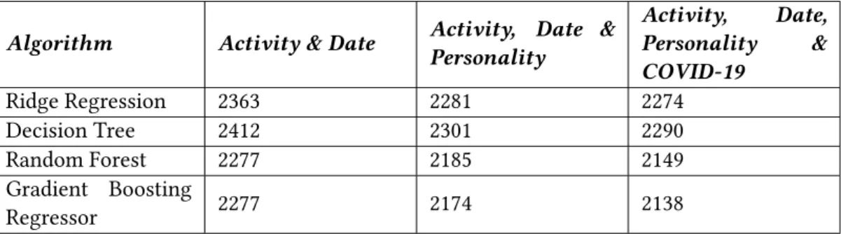
The train set is 90% of the original data set and the remaining 10% is the test set. Tables 5.2 and 5.3 below summarize the results of the 4 ML models for different data sets for the MAE and MAPE metrics, respectively. The performance of the algorithms on the test set for the MAE and MAPE metrics is similar to CV, a fact that indicates that our models were not over-fitted to the training data.

58 For the best-performing data set, the one that includes all activity, personal, and contextual features, we present the performance of the different algorithms in a bar graph format in Figure 5.1.

Table 5.2: MAE for datasets with different feature-groups (training set)

Outlier Handling

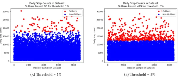
60 approach of identifying and removing outliers on the performance of the GBR model, and then the corresponding results of the isolation forest approach will be presented. In the isolation forest approach, the methodology is similar to manual outlier handling. In this section, we presented the results of the experimental process described in 4.2.2, which aims to detect and remove outliers in the data set.

In the next section, we will present the results of the tested dimension reduction methods to determine whether we can further improve the performance of our model.

Figure 5.3: Outlier and non-outlier distribution in dataset for different threshold values

Dimensionality Reduction

In the following subsection, we will experiment with another approach to reduce the dimensions of the dataset, the dimensionality reduction with PCA. In its algorithmic implementation, PCA requires the user to define the number of components, i.e. the dimensions of the dataset to be created. In Table 5.8 below, we compare the best performances of the RFE and PCA approaches for dimensionality reduction of the data set used.

In Figure 5.9 below, we present a comparison of the different dimensions of the dataset, among others with the performance of dimensionality reduction approaches.

Table 5.7: MAE & MAPE values for the dataset obtained with the RFE approach

Obtaining Optimal Window Size

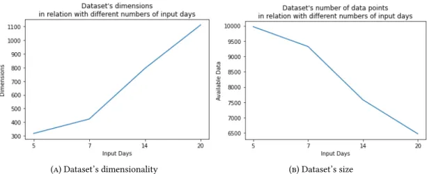
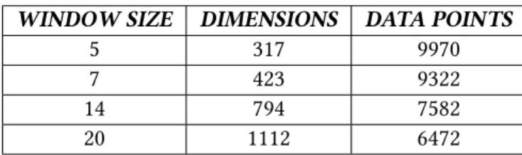
In Table 5.9 below, we present the number of features and the available data points of the dataset, relative to each of the above window sizes. In Figure 5.11 below, we present the values of the MAE and the MAPE metrics obtained by our evaluation process in relation to the different window sizes tested. As already discussed in 4.6 and now clear from the graphs above, there is no significant impact of the window size on the performance of the prediction models.

The given results indicated that there was no significant difference in the performance of the models with respect to the number of input days and therefore we decided to use the window size of 5 days for the sake of efficiency and performance described above.

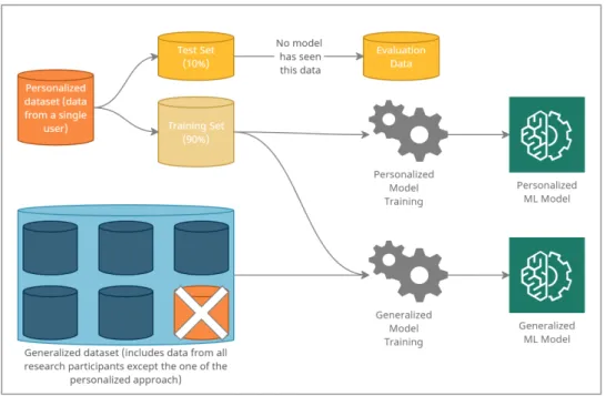
Table 5.9: Dimensionality and available data of the dataset in relation with the window size value.

Generalized and Personalized Model’s Performance

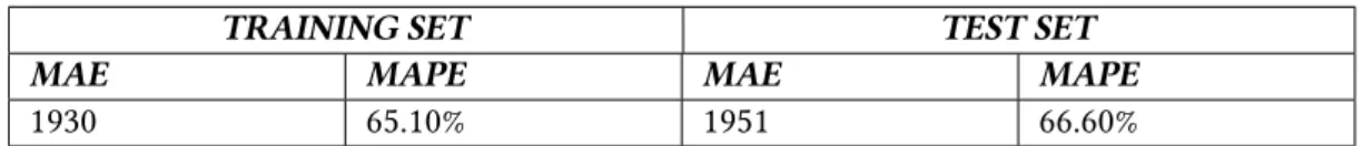
Through this experimental process, we aim to assess the performance of the generalized and the personalized models in predicting a user's future daily step count. In Table 5.10 below we present the values of the two metrics used in the evaluation process. The MAE and MAPE metrics of this approach are shown in Figure 5.15 below, compared to the MAE and MAPE of the personalized model.

In the next section, Section 5.4, we presented the results of two tested approaches to reduce the dimensionality of the data set.

Figure 5.12: Outline of the personalized vs generalized approach.

Demographics Questionnaire

Personality Questionnaire IPIP

Questionnaire of Transtheoretical Model of behavior change

2 - requires closure (only some levels or categories, eg only high schools or just public schools) 3 - requires closure of all levels Blank - no data. 3 - require closure (or work from home) for all-except essential workplaces (eg grocery stores, . doctors) Blank - no data C2 Flag. 1 - recommend closure (or significantly reduce the amount/route/. means of transport available) 2 - require closure (or ban most citizens from using it) Blank - no data.

Individual differences modeling: a case study of the application of system identification to personalize a physical activity intervention. Journal of Biomedical Informatics79 (Mar.