67 Table 5.3a One-step-ahead (h=1 month) out-of-sample prediction accuracy: Modified Diebold-Mariano test and Theil's U. 70 Table 5.3c Twelve-step-ahead (h=12 months) out-of-sample prediction accuracy: Modified Diebold-Mariano test and Theil's U.
Introduction
- The Framework
- Purpose and Research Questions
- Energy Markets
- Energy Products as Physical Commodities
- Properties of Energy Markets
- Energy Futures Contracts
- Outline
On the contrary, the informational content of the remaining economic risk factors included in the economic models is not useful enough to predict expected future returns. Chapter 4 then provides a brief description and analysis of the data series that will be used in the study.
Literature Review
First Stream of Literature: The Two Traditional Theories
4 Positive risk premiums for commodity futures mean that futures prices are initially set lower than the expected future (spot) price of the underlying commodity. The “backwardation” therefore arises as a result of the convenience yield levels and the subsequent negative relationship with the physical inventory levels (Haase and Zimmermann, 2013).
Proposed Economic Predictors
- Predictors of Commodity (Spot and Futures) Markets
- Short-Term Real Interest Rates
- Default Spread
- Term Spread
- US Exchange Rates
- Financialization of Commodities
- Emerging Economies and Global Economic Activity
- Predictors of Traditional Asset Classes
It is because of the stability of the US economy along with the depth of US financial markets (Mileva and Siegfried, 2012). Ravazzolo and Vespignani (2017) also demonstrate strong evidence of their index's predictive power over crude oil prices.
Common Latent Factors
With regard to the second most prominent asset class, namely the bond, the variables that have been empirically shown to have significant predictive power over bond returns, both in and out of sample, have already been discussed in previous sections. To this end, we highlight some alternative approaches. 2016) attempt to empirically study the predictability of expected invoice revenues in an out-of-sample analysis. To account for time-varying potential factors, they use Fama-Bliss forward spreads, forward rates and a latent macroeconomic factor extracted based on the methodology of Ludvigson and Ng (2009); Ludvigson and Ng had also extracted some latent factors to investigate the predictability of bond excess returns.
Regarding the first string, Chantziara and Skiadopoulos (2008) use joint PCA over the period 1993-2003 and derive three (3) PCs from the daily changes in futures prices. They provide evidence that the second PC possesses significant predictive power over changes in heating oil and gasoline prices. In contrast to Chantziara and Skiadopoulos, they find significant evidence of the predictability of oil futures from the first PC derived for any given maturity.
Regarding the second string, Ludvigson and Ng (2009) and Gargano et al. 2016), among others, collect 131 monthly macroeconomic series from the Global Insight database and derive eight (8) common latent factors to predict bond risk premiums. Similarly, in an attempt to analyze oil prices, Le Pen and Sévi (2011) derive nine (9) common latent factors from a large dataset consisting of 187 real and nominal macroeconomic variables such as both developed and developing economies.
The Dataset
- Energy Futures Prices
- The Dataset
- Data Characteristics
- Economic Predictors of Energy Futures
- Economic Predictors
- Data Characteristics
- Descriptive Statistics and Stationarity Tests
- Principal Component Analysis (PCA) Dataset
- McCracken and Ng’s Dataset
- Principal Components (PCs) Characteristics
- Stability of the PCA results
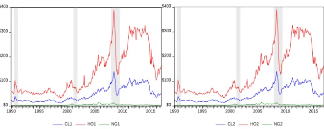
Correlation matrix of the first three shortest and simultaneous futures contracts on the NYMEX WTI Crude Oil, Heating Oil and Natural Gas. 35 We therefore continue by presenting the descriptive statistics for the end-of-month settlement prices of the NYMEX WTI Crude Oil, Heating Oil and Natural Gas futures contracts and the economic variables as well. The evolution of the economic predictors sampled on a monthly frequency is shown in Figure 3.4.
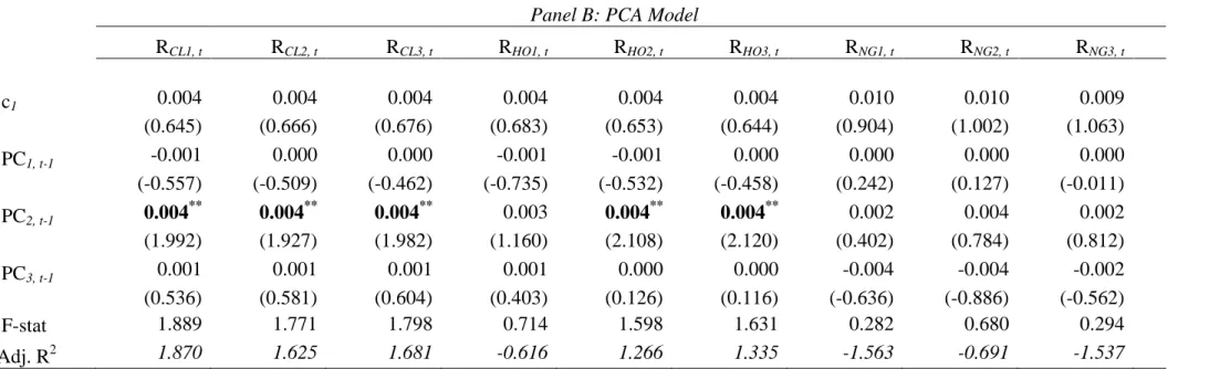
Descriptive statistics of the three shortest maturity futures contracts and economic predictors in levels and first differences. This table reports robustness test regarding the stationarity of the economic predictors sampled at monthly frequency over the in-sample period. Descriptive statistics of the three standardized PCs retained from the Joint PCA and cumulative proportion of variance explained.
Panel B reports the cumulative proportion of original database variance explained by the retained PCs. Panel B reports the cumulative proportion of the variance of the original database explained by the retained PCs for each sub-period.
Methodology
In-Sample Return Prediction Models
- Economic Variables Model
- Univariate Autoregressive Models AR(1)
- Principal Components Analysis (PCA) Models
- Description
- PCs as Predictors – Joint PCA Models
- In-Sample Evaluation Criteria
21 The set of potential predictors may incorporate exogenous explanatory factors along with lagged values of the dependent variable. The PCs are arranged in such a way that the first pairs retain most of the variation found in the original data set. Furthermore, the extracted PCs are able to explain 100% of the variance of the original data set and are arranged in order of decreasing variance.
In this way, the first PC (denoted 𝑃𝐶1) forms a linear combination of variables and accounts for the largest percentage of variance of the original 𝑛 variables. Then the sum of the variances of the 𝑛 PCs is equal to the total variance of the original 𝑛 variables. However, a general rule of thumb suggests retaining the number of PCs that account for 90% of the total variance (i.e., the cumulatively explained variance).
Regarding the sample predictive ability of each factor, we examine the t-statistic and 𝑝-value of the corresponding estimated coefficient. R-coefficients reflect the proportion of the total sample variance that is explained (determined) by the explanatory variables included in the chosen model specification.
Out-of-Sample (OoS) Forecasting Models
- Forecasting Models
- Out-of-Sample Evaluation Criteria
- Standard Performance Measures
- Test of Equal Predictive Accuracy
In other words, the start date is fixed (anchored at the beginning) and the window size grows as we move forward in time; each observation that becomes available (known) is added to the sub-period in the sample and taken into account during the model re-estimation. By repeating this process until the end of the OoS subperiod, we ultimately create a series of P=156 OoS point forecasts of future returns. Let {R̂iT,jt:t+1}t=1P and {𝑅𝑡:𝑡+1𝑖𝑇 }𝑡=1𝑃 denote the order of the one-step-ahead point predictions and the order of the corresponding actual returns over the entire OoS subperiod, respectively.
It is calculated as the square root of the mean squared deviations of model-based return forecasts from actual future returns (Chantziara and Skiadopoulos, 2008). The MAE represents the average of the absolute differences between model-based return forecasts and actual forward returns. A ratio lower than one (<1) indicates a better prediction performance in favor of the first mentioned model.
Then, the statistical significance of the difference between the benchmark and the loss function of the competing 𝑗th model is assessed based on the modified Diebold-Mariano (hereinafter MDM) test proposed by Harvey et al. 23 An alternative method to determine the statistical significance of the OoS -results of the above-mentioned metrics would be the 𝑡-statistic of Clark and West (2007) (see Gargano and Timmermann, 20014).
Empirical Results and Discussion
In-Sample Evidence
Regarding the default spread, our findings are consistent with Bessembinder and Chan (1992), who find limited predictive power of the junk bond premium in 12 futures markets. On the other hand, we find negative but insignificant results in the case of natural gas profits. Regarding this finding, we assume that this is a consequence of the costs of natural gas storage.
Although the lagged values of the second principal component (PC2) are found to be statistically significant for WTI crude oil and fuel oil futures, the results indicate an overall poor fit of the PCA model; The F statistic indicates that the PCs are unable to predict the expected future energy returns. In particular, the following specification is estimated by Ordinary Least Squares (OLS): 𝑅𝑖,𝑡 = 𝛼0+ 𝑎1 𝑜𝑖_𝑔𝑟𝑡−1+ 𝑎2 𝑑(𝑡−1)𝑡−1 𝑠)𝑡−1+ 𝑎4 𝑑(𝑑𝑓𝑠)𝑡−1+ 𝑎5 (𝑡𝑤𝑑𝑖)𝑡−1+ 𝑎6 𝑑(𝑙𝑤𝑠𝑝)𝑡−1+ 𝑎7 𝑅𝑀,𝑡−1,𝑡− 𝑖-th commodity futures monthly prices, log-difference, 𝑜𝑖_𝑔𝑟: the median open interest rate growth for all the underlying assets studied, 𝑑𝑖𝑟: the changes in the short-term real interest rate, calculated. The above specification OLS estimates of the parameters along with their corresponding t-statistics in parentheses, the adjusted R2 and the F-statistics are also reported in the table.
The OLS estimates of the parameters according to the above specification, together with the corresponding t-statistics in brackets, the adjusted R2 and the F-statistics, are also reported in the table. The OLS estimates of the parameters in the above specification, along with the associated t-statistics in brackets, and the adjusted R2 and F-statistics, are also reported in the table.
Out-of-Sample Forecasting Performance
Nevertheless, these findings are in sharp contrast to the Theil's U results for the OoS performance of each predictive model. For the forecast period of one, three and twelve months (ℎ=1,3,12), the table reports two ratios based on the out-of-sample (OoS) measures of the three forecasting models used in the context of this study, viz. For each of the recursively estimated predictive models, metrics were calculated over the OoS subperiod (ie, Jan 2004–Dec 2016).
The MDM test based on the mean loss differential (i.e. the squared error and absolute error in panels A and B respectively) and the Newey-West estimator of the standard deviation 𝑑̅̅̅̅̅̅̅𝑡+1|𝑡𝑖𝑇,𝑗 examines the null hypothesis (H0 ) against two alternative hypotheses, H1 and H2. For each of the recursively estimated forecast models, metrics were calculated for the OoS sub-period (i.e. January 2004–December 2016) for a forecast period of one month (ℎ=1). For each of the recursively estimated forecast models, metrics were calculated for the OoS sub-period (ie, January 2004–December 2016) for a forecast period of three months (ℎ=3).
72 tial (i.e., squared errors and absolute errors in panels A and B, respectively) and a Newey-West estimator of the standard deviation of ̅̅̅̅̅̅̅𝑡+1|𝑡𝑖𝑇,𝑗 the two alternatives (H0ll) examining the two alternatives (H21 hypotheses, H0ll) . For each of the recursively estimated predictive models, the metrics have been calculated over the OoS sub-period (ie Jan.2004-Dec.2016) for a forecast horizon of twelve months (ℎ=12).
Conclusions and Implications
For seven of the nine future scenarios examined, the economic models appear to satisfactorily meet the associated returns. U from the AR(1) models for the forecast horizon of ℎ=1 month, we conclude that the out-of-sample predictability becomes stronger as the duration of the respective futures contract increases. Journal of Economic Perspectives 18 (4), pp. https://wwz.unibas.ch/fileadmin/wwz/redaktion/makroekonomie/intermediate_macro/re ader/9/02_R_Oil_and_the_Macroeconomy.pdf. 2017) ‘A stochastic supply/demand model for storable commodity prices’.
Commodity Prices and Markets, East Asia Seminar on Economics 20, pp. 2008) 'Can the dynamics of the term structure of petroleum futures be predicted. 2010) ‘Can Exchange Rates Predict Commodity Prices?’. American Journal of Agricultural Economics 66 (5), pp. https://sites.hks.harvard.edu/fs/jfrankel/commodityprices.pdf. 2006) 'The Effect of Monetary Policy on Real Commodity Prices'. 2014), 'Effects of Speculation and Interest Rates in a "Carry Trade" Model of. International Journal of Finance 13 (2), pp. 2012) 'What do futures market interests tell us about the macro economy and asset prices?'. 2009) 'Not all oil price shocks are the same: Disentangling demand and supply shocks in the crude oil market'. http://www-personal.umich.edu/~lkilian/aer061308final.pdf. 2017) 'How the Tight Oil Boom Changed Oil and Gasoline Markets'.
Journal of Banking & Finance 84, pp. 2015) ‘Robust Econometric Inference for the Predictability of Stock Returns’. 2016) Common factor 'commodities': an empirical assessment. What is the role of the United States?'. 2016) ‘A new monthly indicator of global real economic activity’.