2.1 Structural Health Monitoring

The new generation of smart devices has a variety of sensors that can be used to build scalable and extensible surveillance systems with hundreds of nodes. In this paper, we present a distributed mobile structural health monitoring (SHM) system using smart handheld devices. We describe a distributed clustering algorithm that gathers nodes that produce similar power spectra and thus enables the implementation of decentralized heavy computation algorithms that operate on the power spectrum of the collected sensor values.

This report is my Master's thesis for the completion of my postgraduate studies at the Department of Informatics and Telecommunications, University of Athens. It was developed as part of my work in the KDD lab of the MadGik research group.

Introduction

By using MSNs instead of WSNs, we can reduce infrastructure costs by incentivizing smart device owners to contribute to the purpose of the MSN, making their smartphone or tablet a discovery node of the MSN. Two of the main advantages of smart devices are their computing capabilities and their storage. In addition, the cost and size of high-precision acceleration sensors are expected to continue to fall, so it's safe to expect smart devices to include the latest sensors in the near future.

We propose a distributed clustering algorithm that groups nodes that produce similar power spectra and thus enables the implementation of decentralized heavy computation algorithms that operate on the power spectrum of the collected sensor values. We describe a scalable, fault-tolerant communication protocol, which performs the best time synchronization of the nodes, which is necessary for accurate SHM.

Related Work

Structural Health Monitoring

Related work

Results were evaluated against theoretical models and previous bridge studies and synchronization and jitter issues were addressed. The focus of this work is to minimize the communication cost between WSN nodes and maximize energy efficiency. Our system can be extended to accommodate more sophisticated operational modal analysis techniques that are based on structure acceleration sampling.

In other words, a single node on the network was unable to determine which features to monitor based solely on the node's own data. Based on that, the quality of SHM with smart devices, which serves as the application and evaluation domain of our algorithms, depends only on the performance of the embedded accelerometer.

Problem Description

Our proposed distributed framework performs a hash-based clustering on an approximation of the observed power spectra. Next, the clustered nodes exchange their power spectra to find their nearest nodes and finally the nearest nodes contribute to the system's goal. Our approach extends the current existing works by accommodating the state-of-the-art SHM algorithms and techniques on smart handheld devices, such as smartphones and tablets.

This approach breaks the barrier of the limited number of sensors currently deployed, therefore it can enable the deployment of SHM applications in buildings consisting of tens of floors. Furthermore, the installation costs of SHM deployments are drastically reduced because the sampling hardware needed by SHM applications is already carried by the people who already occupy the building and as a result, their smart devices replace the expensive dedicated sensors that are currently used. Moreover, the existence of a central server that was previously used to collect and analyze the data from the installed accelerometer sensors does not exist in our architecture.

Communication Protocol

Communication Protocol

• Bootstrapping and nodes joining the MSN
• Detection of fallen nodes
• Clustering of nodes with similar power spectra

This ∆t is minimized by repeating the above procedure, until the calculated difference converges and does not change significantly. When the initialization procedure is complete, the new joining node s receives a PEER-DATA message from the master node m, describing the state of its peers and previous system exits. Peers' state currently includes their IP addresses, but it could be expanded to accommodate more data, depending on the experiment MSN intends to perform.

Periodically, all nodes send a HEARTBEAT message to the master node every Tp second to indicate that they are still contributing to the experiment. If the node does not receive a HEARTBEAT message from the nodej for a period of several seconds, the nodeji is considered down and its error is broadcast to the network for the rest of the peers to remove its IP address from their peer data , received by the PEER -DATA message when they joined the system. If the current master node m is detected as down via HEARTBEAT's socket connection, the node with the lowest local IP address is immediately selected as the new master in the network without further communication.

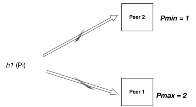
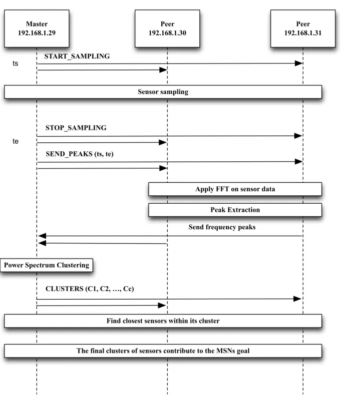
The master node mudsends an on-demandSEND-PEAKS message to its peers to collect their power spectrum peaks. When a node receives a SEND-PEAKS message, without stopping the procedure of collecting sensor data, it computes the Fast-Fourier Transform (FFT) [4] of its collected sensor time series and then selects ns frequency-height pairs, as described in Sect. 6 , corresponding to its power spectrum peaks. The master node, after collecting peaks, applies PowerHash Clustering, described in Section 4.1, to group nodes with similar power spectra and broadcasts a CLUSTERS message containing the created clusters, C1, C2,.

After collecting the CLUSTERS message, MSN nodes exchange their power spectra within their cluster to find their nearest nodes, and then start communicating with their best matches to contribute to the MSN goal.

Clustering Algorithm

Power Spectrum Hash-Based Clustering

• Definitions
• PowerHash Clustering Algorithm

Therefore, we amplify the information these peaks provide by including the relative frequency and height distances of the successive peaks in our hash function. Near average value of their Relative Frequency Distances 5. Near average value of their Relative Height Distances. How close the last four values ​​of the attributes will be is defined by the twoGranularity parameters.

Peak Extraction: Each sensor-enabled node divides its power spectrum into wavelength chunks. and finds the maximum peak within each slice. They should differ in frequency distance a percentage of the total length of the power spectrum as the node, which can be set by the domain expert, according to the nature of the application domain. After filtering, the remaining peaks will be used to describe the power spectrum of the sample sensor data. fnsi, ansi)}, where (fj, aj) represent the frequency and height of the jth peak, respectively.

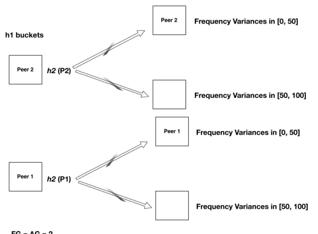
Data aggregation: Each sensor-enabled node sends its calculated power spectrum peaks, frequency pairs and values, to the master node m, selected by the process described in section 3.1. In this step, E(F(si)) and the maximum relative frequency distance average, RF DAmax, are stored for calculation of equation 4.6. Let A(si) be the discrete random variable representing the relative height distances of node si.

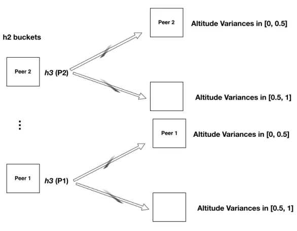
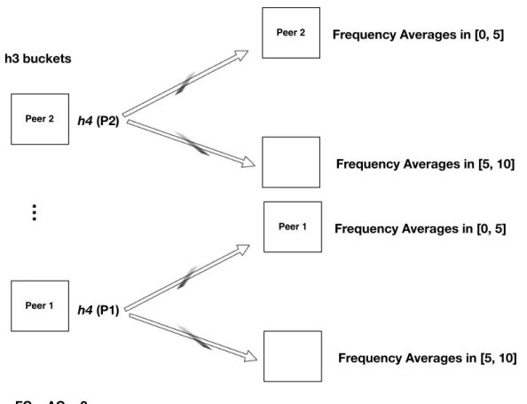
In this step, each sensor's average peak relative height distance, E(A(si)) and average maximum relative height distance, RADAmax, are stored for the calculation of Equation 4.7. Computation RF DAmax−RF DAminc (4.6) h5: This step divides the possible values ​​that E(A(si)) can take into ranges and assigns E(A(si)) to the corresponding range. E(A(si)) and RADAmax are pre-calculated by calculation step h3. Hash Aggregation: For each sensor si, the master node calculates the P owerHash value H(si), described in Algorithm 6, which combines the precomputations1(si),h2(si),h3(si),h4(si).

Experiments

• Experimental Setup
• Distances of the nearest intra-cluster and nearest inter-cluster sensorssensors
• Spatial Discovery

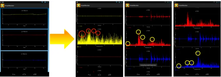
The average value of the results for each different AG value formed the result of the FG Constant experiment. Our data turned out to be more sensitive to the AG parameter, which can be explained by the very similar frequency bins of the power spectrum peaks, shown in Figure 5.9, that our data set had. We measured that the average number of peaks extracted for all our experiments was 0.09765% of the total length of the power spectrum, which means that on average, 4 peaks were extracted from the 4096 points of the power spectrum.

To see the effect that the presented excitation had on the relative distances of the produced power spectrum time series of the sensors, we applied the following distance metric. Where si(f) and sj(f) are the height of the f-th frequency bin for sensors si and sj. Figure 5.3 shows the values ​​of the average value of the distances of equation 5.1 for the three different excitation levels and the two structure conditions.

We observed that for the undamaged state, the higher excitation decreased the distances of the respective power spectrum time series, while in the damaged state it increased. In addition, the state of the structure influenced our results, increasing the distances as the excitation level increased for the damaged state and improving the distances as the excitation increased, for the undamaged state. As explained in section 1, the goal of our method is to group sensor-driven nodes with respect to the power spectrum of the collected acceleration data.

For the damaged condition, the higher the arousal level, the lower the performance of the spatial detection score. Note that in the figure the position of the plate sensors is lower than the actual position, for visual simplicity. As a result, we run our clustering algorithm without the datasets from the second floor, and PowerHash Clustering kept the two floors in different clusters.

Due to the effect that the state of the structure had on our experiments, we performed intercondition experiments, combining sensor data sets from the intact and the damaged state of the structure, aiming to create clusters that captured the state of the structure. . Each clustering was evaluated as the percentage of clusters that consisted of more than one sensor and included only sensors from the same condition.

Conclusions

Appendix A

Power Hash Clustering Core Source Code

42 grup statik publik HashMap> (int fg, int ag, ArrayList> nodePeaks).