The first experimental observation of the SM Higgs boson took place on 4 July 2012. Furthermore, the coupling of the SM Higgs boson to fermions is of the Yukawa type and is therefore expected to be proportional to the fermion's mass. One of the most recent discoveries confirming the Standard Model was the first experimental observation of a particle with a mass around 125 GeV compatible with the SM Higgs boson (July 4, 2012)[1,2].
Particles and Interactions of the SM
Particles of the SM
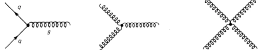
It provides a unified description of the particles that make up matter, in which forces are mediated by the exchange of particles. The first type corresponds to bosons that act as mediators of various forces while the second type is responsible for giving mass to particles through the Higgs mechanism and is called the Higgs boson. The gauge bosons that act as mediators of fundamental interactions (Table 2.1) are gluons (g), photons (γ) and W± and Z0 bosons respectively, while the graviton, the so-called mediator of gravity, has not been observed. .
Interactions of the SM
The color charge of the particles can be red, green or. a) Fundamental quark-gluon peak of QCD. Asymptotic freedom As can be seen in Figure 2.4, when the energy rate Q increases, the value of the coupling constant α decreases. In the following equations we can observe the currents of weak isospin triplets and the corresponding algebra they obey.
The Higgs Mechanism
It is defined with respect to the electric charge according to equation (2.8), where T3 is the third component of the weak isospin T. The Lagrangian describing the SU(2)L×U(1)Y gauge symmetry group of the unified electroweak interactions. LEW =Lgauge+Lf+LHiggs+LY uk (2.9) where LEW describes the interactions between the B and W bosons, Lf is the fermion term, LHiggsis is the Higgs part of the Lagrangian and LEWY uk is the Yukawa interaction term.
The Higgs boson
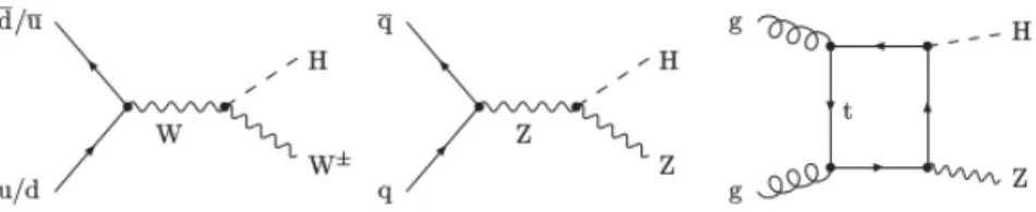
Higgs production processes
Gluon fusion Gluon fusion through a heavy quark loop (b or t quarks) is the most dominant production mechanism of the Standard Model Higgs boson in hadron colliders. The main contribution comes from the top quark, due to the large Yukawa coupling it has to the Higgs boson. This production mechanism is a direct probe for measuring the Yukawa coupling of the top quark and Higgs boson.
Higgs Decay processes
The total decay width and the branching ratios of the SM Higgs boson as a function of the Higgs boson mass are shown in Figures 2.11 and 2.12. For the Higgs boson with a mass value of mH = 125GeV, the total decay width has an order of ≈4 MeV.
The top quark
Top quark production
In strong interactions, the top quark appears as an at¯tpair, and in weak interactions as a single top quark. The cross section for the production of a pair of top quarks can be written in the following form, where i,j are the input partons, which can be gluons, valence quarks or sea quarks, h1. In Figure 2.14 we can see a schematic view of the production of this pair, while in Figure 2.13 we can see the Feynman diagrams of leading order contributions to this particular process.
Top quark decay
Therefore, the measurement of top quark polarization and spin correlations is performed by studying the angular distributions of various decay products.
Parton distribution functions in pp collisions
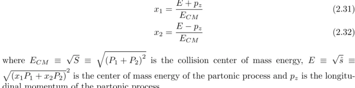
P1+P2)2 is the collision center of mass energy, E ≡ √ ˆ s ≡ p(x1P1+x2P2)2 is the center of mass energy of the partonic process, and pz is the longitudinal momentum of the partonic process. They must therefore be normalized in a way consistent with the quantum number of the proton. The first number below each ring represents the date it began operating. The number in parentheses represents the size of the ring.
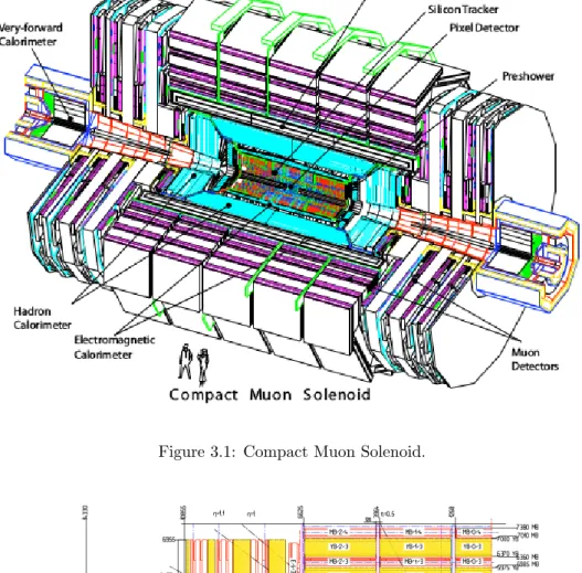
The Compact Muon Solenoid
- Coordinate System
- Magnet
- Muon System
- Electromagnetic Calorimeter
- Hadron Calorimeter
- Inner tracking system
- Trigger
In Figure 3.2 we can see a quarter cross-sectional view of the CMS experiment with some dimensions and lines of constant η superimposed[21]. The flux of the magnetic field is returned by 10,000 tons of iron yoke. The yoke consists of 5 barrels and 2 end pieces of 3 layers each. In the barrel region (|η| < 1.2) the neutron-induced background, muon velocity and chamber residual magnetic field are low.
In contrast, in the two end caps (1.8<|η|<2.0), the neutron-induced background, muon rate, and magnetic field are high. Evaluation of the energy resolution of the ECAL supermodule was performed using a test beam from the LHC. We can see all four components of HCAL: the hadron barrel (HB), the hadron hood (HE), the outer hadron calorimeters (HO) and the hadron forward calorimeters (HF) [26].
In Figure 3.10 we can observe the Jet transverse energy resolution as a function of the simulated jet transverse energy for the three hadron calorimeter regions. There are 3 additional inner discs in the area between the barrel and end cap parts, on each side of the inner barrel. The choice of the trigger paths defines which physics objects must be found to accept the event.
The first two equations refer to the missing transverse energy of the x (Ex) and y (Ey) axis.
Analytical solution
Finally we have managed to reduce the initial system of equations to a system of two equations with two unknown variables, which is solvable. Finally, the resultant can be obtained by calculating the determinant of the following Sylvester matrix which equals zero. The above resultant corresponds to the following univariate polynomial which contains only the remaining unknown variable pvx.
For the purpose of this thesis, we consider in all equations described in this section that the neutrino and antineutrino masses are equal to zero.
Model independent mass reconstruction
- Method description
- Method performance
- Solution selection
- Optimization of m top and m W constrains
- Parton interactions and PDFs
- Signal Samples
- Background Samples
Of these objects, two out of four b-jets originate from the decay of the Higgs boson, while the remaining objects originate from the t¯t decay process. For each event, two of the four b-jets are attributed to the Higgs boson and the remaining two to the t¯t system. In contrast to this improvement, the shape of the Higgs mass distribution shown in Figure 4.7 remains roughly the same.
In Figure 4.10 we can see that the shape of the Higgs mass distribution is similar, but the peak is amplified. When using the maximum weight solution selection, the method can correctly reconstruct approximately 35% of events with respect to the mass value of the Higgs boson. We can ultimately conclude that the choice of the maximum weight solution is the most efficient and will be used in all subsequent studies for the purpose of this thesis. a)mtopdistribution of all solutions yielded by the method. b) mW distribution of all solutions produced by the method.
As we can see in Figures 5.4 and 5.6, the shapes of the Higgs mass distribution when using a bounded and unbounded topandmW mass cycle shape are similar with respect to the low- and high-mass tail. In this case, the method is able to correctly reconstruct approximately 43% of the events regarding the Higgs boson mass value. As a result, choosing the limits mtop GeV and mW ∈[60,100] GeV increases the efficiency with respect to the peak in the Higgs mass distribution, and for the purpose of this thesis, will be used in all the following studies.
In the next section, we will repeat the steps leading to the reconstruction of the Higgs boson mass, this time using MC reconstruction level events that resemble the signal and the backgrounds of this particular process.
Pre-selection Criteria and event yields
Sanity check
To cross-check our code, ntuple production, and resulting event yields, we compare the resulting event yields with the HIG-16-038 analysis using the same preselection given in Figure 5.14 [34]. The event yield of the two analyzes and their relationship can be seen in table 5.3. The second column corresponds to the event yield calculated for this thesis by reproducing the HIG-16-038 analysis event selection, while the event yield in the third column is taken from the HIG-16-038 analysis and scaled to 200f b−1 .
According to the last column of Table 5.3, we were able to reproduce the HIG-16-038 assay event yields within approximately 15% agreement. After this short sanity check, which ensured the validity of our code, n-fold production, etc., we will proceed to extrapolate the event yields for a luminosity of 200f b−1 using the optimized preselection discussed in Section 5.2.
Event yields
According to the resulting yields forLumi= 200f b−1 we expect 50 signal events compared to about 1200 background events. As expected, the most dominant background is the t¯t+jets process, which accounts for approximately 97% of the total background.
Higgs mass distributions
Optimization studies
Data-driven background estimation
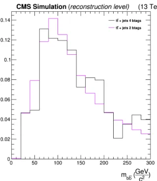
So we will use this sample to predict the background shape of the t¯t+jets process when we request four b-labeled jets. The signal shape of the t¯tH, H →b¯b process corresponds to the shape of the four b-tag claims, whereas the shape of the t¯t+jets background is extrapolated from the two b-tag states , scaled to the number of expected events when requesting four b-tags. The scaling factor for the →b¯b background from two to four b-tags is taken from the MC studies and corresponds to 0.0044.
Finally, it is reasonable to calculate significance near the peak. Finally, in Figure 5.15(c) the distributions of the quantity log10(x1x2) are also different, a fact that we expected due to the different final states of the signal and background processes. The first column corresponds to the absolute number of events that pass event selection (L= 12.9f b−1), the second column corresponds to the number of MC events that pass event selection, scaled by data brightness, and the third column, which is the ratio of the first two, corresponds to the k-factor of the HIG-16-038 analysis.
The fluctuations are due to the low statistics of the Data sample, which after event selection had an event yield of ~300 events. In the left figure we can observe the mb¯b data distribution with black points superimposed on the corresponding MC distribution (red line) adjusted to the data luminosity, L= 35.9f b−1, where the x-axis has been magnified. In the right picture we can observe the relationship of the data over the MC events. a) DR between two b jets assigned by the method to the Higgs mass reconstruction.
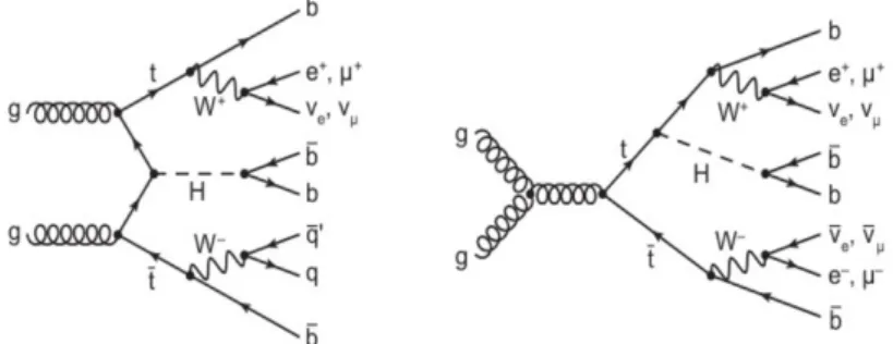
The study of concomitant production of a Higgs boson and a t¯t pair is essential, as it is a direct investigation of the measurement of the top Higgs Yukawa coupling. Also, a data-driven estimation of the background shape as well as scale factor will be performed, using the Tagging Rate Function (TRF). 2] ATLAS collaboration, “Measurement of the Higgs boson mass from the H →γγ and H →ZZ∗→4` channels with the ATLAS detector using 25 fb−1ofpp collision data,”.