Subspace Clustering: A Possibilistic Approach

The main issue in the clustering problem is defining the relationship of a data point to a cluster. In the subspace clustering concept, dimension reduction methods are used to estimate the dimension of the subspaces involved.

Principal Component Analysis (PCA)

Statistical view of PCA

Therefore, the direction along which the data exhibits maximum spread is the eigenvector iΣX,uˆ1 associated with its largest eigenvalue. It is desirable that the second principal component be uncorrelated with the first, which is Corr(y2, y1) = 0⇔ Cov(y2, y1).

Geometric view of PCA

2.1.22 we conclude that the objective function obtains the maximum value for the matrix Uˆ whose columns are the eigengene. These eigenvectors are the upper left singular vectors of X∗, which are equivalent to those obtained by the classical PCA approach in Section 2.1.1.

Alternating Iteratively Reweighted Least Squares (AIRLS)

Hopefully, the cardinality of the remaining columns will be equal to the true dimension of the subspace. Subspace clustering refers to the clustering problem where data are distributed across different subspaces of ambient space1.

K­Subspaces clustering

Note that forK = 1 the problem becomes that of geometric PCA, while fordj = 0, there are no bases and projections (respectively {U}Kj=1,Yj), so the algorithm becomes that of Kmeans. The latter occurs when the data instead of flat-shaped clusters form compact and hyperspherical-shaped clusters. The algorithm gradually evolves as it tries to approach a local minimum of the cost function in 3.2.1.

As one can easily observe, the major problem with Ksubspaces is that the number of apartments and their dimensions must be known a priori, a matter that is hardly met in practice.

RANdom SAmple Consensus (RANSAC)

The procedure ends by returning the evaluation of each subspace (cluster) of the set of inliers and reassigning each point to its nearest cluster. It is extremely stable to externalities and the number of subspaces K need not be known a priori. Its main disadvantage is that the probability of getting a large number decreases exponentially with the number of subspaces.

Consequently, the number of maximum iterations must become larger as the number of subspaces and their dimension increases. In cases where the dimensions differ, subspaces can be evaluated in ascending or descending order of dimensions. If we start by estimating the subspace with the highest dimension, it is expected to be assigned the data belonging to the subspaces of lower dimension (model overfit).

On the other hand, if one starts with the lowest dimension, the first estimated subspace is very likely to be assigned to data belonging to intersections of subspaces or data belonging to the subspace of the highest dimension.

Spectral Local Best­fit Flats (SLBF)

The process continues with the computation of the diagonal matrix and the normalization of the affinity. Finally, the produced matrix is ​​factorized and Kmeans are applied to the rows of the matrix composed by the top core vectors5 of the normalized affinity multiplied by the corresponding eigenvalue matrix. Note that Kmeans takes as an input parameter the number of clusters equal to the cardinality of the chosen eigenvectors.

However, the complexity of the latest increases as the dimension and the number of clusters increase. Another important advantage of the algorithm is that it automatically determines the size of the neighborhood via algorithm 4. It is clear that since the algorithm works with neighbors, it is expected that outliers will be rejected as they lie far from the region where the majority of the points lie.

In addition, the dimension of the subspaces must be a priori and equal for all subspaces, since a subspace is appropriate to each neighborhood of each point.

Sparse Subspace Clustering (SSC)

Uncorrupted data

Ideally, the cardinality of those nonzero entries is equal to the dimension of the corresponding subspace. Therefore, to limit the number of possible solutions and impose sparsity, the authors in [8] propose to solve the following convex relaxation optimization problem:. This eliminates scale differences between larger edge weights since spectral clustering tends to focus on the larger graph links.

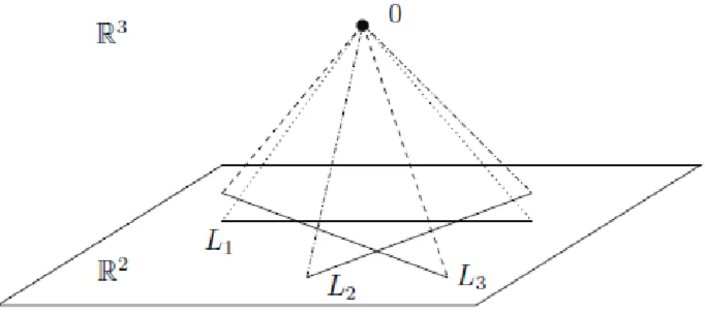
So to fit in an affine subspace d+ 1 points are needed, where d is the dimension of the affine subspace. To illustrate this, as written in [23], imagine the linear subspaces corresponding to the affine lines x= 1 and x=−1. Thus, the number of subspaces is equal to that of the connected components in the similarity graph.

The SSC rationale is also extended to the concept of corrupt data (outliers, noise, large errors and missing data).

Corrupted data

In the context of subspace aggregation, this cost includes the distance of the points from the subspace. It is a measure of the variance of the data points of a cluster Cj around its connected subspace Sj. Only the second term of the cost function contains values ​​of wij in the interval (0,1).

In the following, we explain in detail the main components of the algorithm and their characteristics. We continue to consider the update of the main parameters and the selection of parameters for regulation. We find a neighborhood for this center and estimate the subspace of the corresponding cluster.

The size of neighboring sets of points plays an important role in defining subspaces.

Main processing part

• Segmentation (update of w ij ’s)
• Update of µ j ’s
• Update of U j ’s and Y j ’s
• Cluster elimination and update of η j ’s
• λ 1 selection

To update the displacement vector µj of the subspace Sj, we use the formula derived from the derivation of the cost function 4.0.3 w.r.t. In the following, we show how the method expressed in [10] (see Section 2.2) can be adapted in the context of the present problem to tackle the problem of unknown subspace dimension. Therefore, in order to find cluster membership, we fit the closest cluster to each point.

More precisely, each of the points is assigned to the group for which it shows the maximum degree of compatibility. In this way, only a part of the initial subspaces will be moved closer to the clusters (those that fit better), the rest will fit small groups of points that either lie approximately in the same subspace (coincide) or form clouds noise2. Specifically, a group is eliminated if either its cardinality is less than the dimension of the associated subspace or if the dimension of the subspace is zero.

The latter happens when λ2 shrinks all the columns of the connected matrix to zero, showing that this particular group of points does not extend along any subspace.

Model selection (λ 2 selection)

SAP K­subspaces algorithm

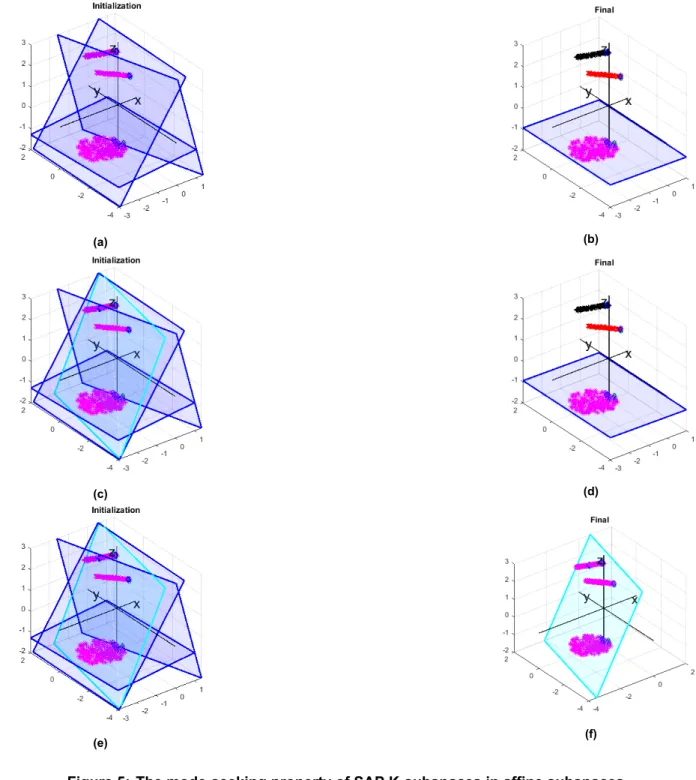
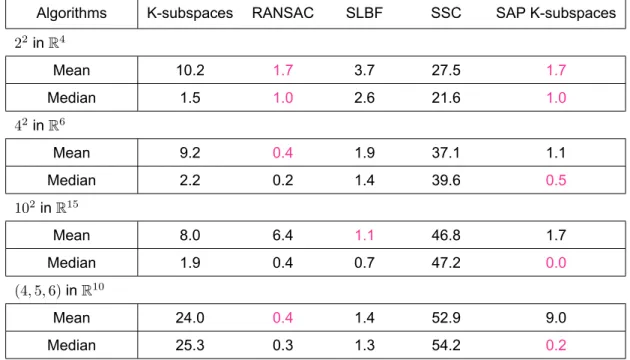
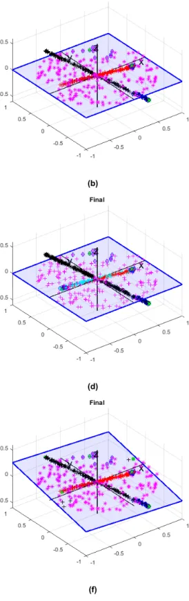
Subspaces are initialized based on the neighborhoods of the most distant points of the dataset (those with the greatest Euclidean norm). RANSAC and SLBF do not support the case where the dimensions of the subspaces differ. In the first part we study the case of the Klinear subspaces and in the second part the case of the Kaffine subspaces.

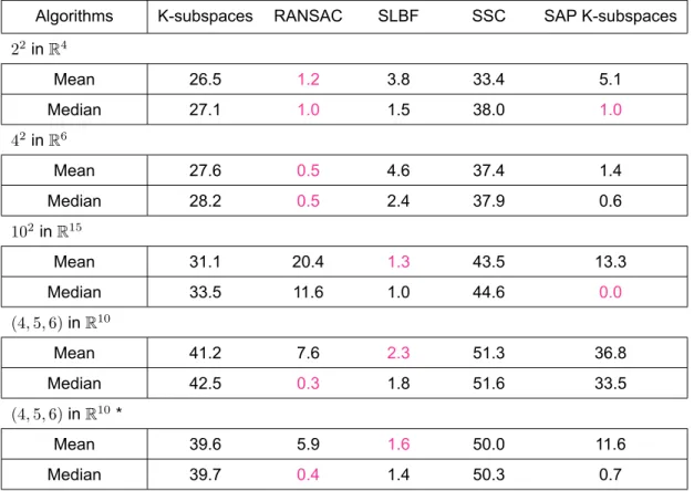
Note that in the Gaussian model, most of the data lies in the intersection of the subspaces. Consequently, we encourage the algorithm to take points from the intersection of the subspaces to evaluate each subspace. As we increase the number of outliers (Tables 2 and 4), Ksubspaces struggles to discover the underlined structure of the data set.

Increasing the number of initial (linear) subspaces using the PFI method allows the algorithm to detect the actual number of clusters.

Clustering results on motion segmentation data

This is because clusters are as a desired condition for SSC that the subspaces are uniformly distributed, independent and disjoint. In the above tables, the parameters (d,p) next to the algorithm name indicate the dimension of the subspace (initial for SAP Ksubspaces)d and the dimension pro. The algorithm is able to estimate the true number of equally populated clusters and the variance and dimension of the corresponding subgroup.

It turned out that the ability of SAP Ksubspaces to estimate the number of clusters is highly dependent on a parameter Ξ that controls the degree of truncation imposed on the degrees of compatibility of a data point with clusters. However, those groups must be of the same size, since the same parameter λ2 is used for each group. When this criterion is met, SAP Ksubspaces shows the best performance in most cases.

Interesting research opportunities include the creation of a scalable, possibilistic subspace clustering algorithm that reduces the size of the subspaces without imposing drawbacks.

Notation

• Sets
• Scalars
• Vectors
• Matrices
• Norms

X ∈RL×N, whose columns are the data vectorsjixi Xj ∈RL×Nj, whose columns are the data vectorsjixi ∈Cj. Yj ∈Rd×N, with the columns of the rectangular projection of the data onto the Sj Im Them×midentity matrix.

Definitions

Linear Algebra

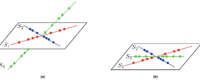
A set of points {xi}Ni=1 is said to be linearly dependent if there are scalarsκ0, .., κN not all zero such that PN. If S has identical definitions of vector addition and scalar multiplication to those of V, then S is called a subspace of V. K linear subspaces of a vector space V are said to be independent if the dimension of their sum is equal to the sum of their dimensions, .

K linear subspaces of a vector space V are said to be disjoint if each pair of subspaces intersect only at the origin.

Affine Geometry

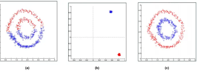
Spectral clustering is a technique suitable for high-dimensional data, and they can reveal clusters of any shape, provided they are not intersected. Basically, what we do with spectral clustering is we map the data into a new space (usually of a lower dimension), where the clusters (hopefully) become compact and hyperspherically formed. Two-dimensional dataset forming two clusters. a) The Kmeans clustering results when applied to the original dataset. b) The Kmeans data is applied.

From the weights of the graph, the matrix A∈RN×N is created, which is called the graph's weighted adjacency matrix, or simply the affinity matrix. In other words, it is an indication of whether the two points should be assigned to the same group or not. However, one can think of the graph Laplacian as a matrix that allows us to perform clustering based on its properties.

Finally, a compact clustering technique is applied to the rows of U (each row corresponds to one data point).

K­Subspaces

RANdom SAmple Consensus (RANSAC)

Neighborhood Size Selection for HLM by Randomized Local Best Fit

Spectral Local Best­Fit Flats (SLBF)

Sparse Subspace Clustering (SSC) for Uncorrupted Data

Sparse Subspace Clustering (SSC) with Outliers

Sparse Subspace Clustering (SSC) for Noisy Data

Sparse Adaptive Possibilistic K­Subspaces (SAP K­Subspaces)