Temporal Abstraction for Hierarchical Reinforcement Learning in Air Traffic Management

We consider the planning of air traffic management operations in the pre-tactical phase: Given air sectors' limited capacity, one of the major issues is to minimize ground delay costs while ensuring the efficient utilization of airspace. A generic hierarchical multi-agent reinforcement learning (H-MARL) method is developed that can operate at various levels of abstraction: It is instantiated to alternative H-MARL methods that exploit different levels of abstraction of the action-state-space with respect to the DCB problem. Hierarchical multi-agent reinforcement learning methods are evaluated in relation to other modern flat models and methods [1].

The duration of each such period shall be equal to the duration of the period used to define the capacity. This information per trajectory is sufficient to measure the demand for each of the sectors R∈R in the airspace during any counting period.

Data Sources

Thus, our work is closer to the first of the aforementioned classes of state abstraction methods, which group states with similar environmental configurations and related behaviors. The time step size determines the amount of time instances that elapse before the action completes. This prunes the states that the agent will explore at the abstract level L, since states with a delay that is not a multiple of the time step are unreachable.

Moreover, we aggregate original (ground) states with delays betweeni∗asL and(i+ 1)∗asL,i∈N, into the same abstract state. The joint statesL,tAg of a set of agentsAg at the time abstraction levelIs the tuple of the state variables for all agents inAg. C(sti, strti) is a function that depends on Ai's participation in hotspots while executing its trajectory according to the strategy strti, and.

We have chosen that C(sti, strti) depends on the total duration of the period in which agents fly over busy sectors. The DC(strti) component of the reward function corresponds to the strategic delay cost when flights are delayed at the gate. In the Independent Reinforcement Learners (IRL) framework, each agent learns its own policies independently of the others and treats other agents as part of the environment.

It should also be pointed out that instead of the global reward Rwd(s,str) used in [7], we use the reward Rwdi received by agentAi, considering only the local state and local strategy of this agent.

Independent Hierarchical Q-Learners

• Descending Timesteps (DT)
• Unitary Timestep, Limit State Space (UTLSS)
• Unitary Timestep, Concurrently Update Levels, Limit State Space (UTCULSS)
• Unitary Timestep, Limit State Space, No Experience Transfer (UTLSSNET)

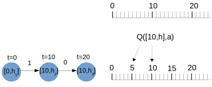
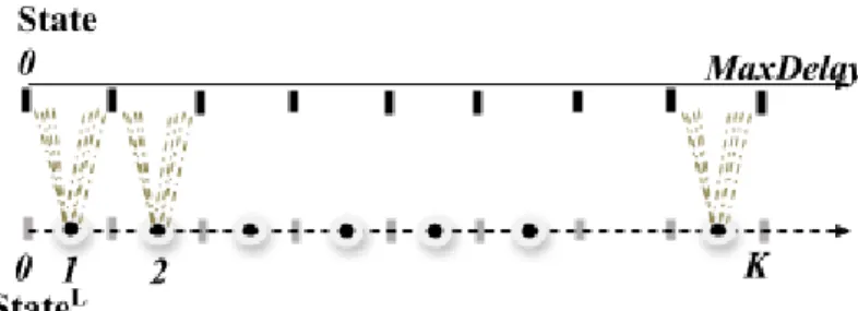
State map to multiple abstract StateL spaces, where |StateL| « |State|.This includes the (original) ground state space abstraction. As described in 6.2b, the Q values ​​of the first ten-minute interval are mapped to the Q values ​​of the first and second five-minute intervals of level 2 w.r.t. hotspots and related actions. Case (a) shows the local state transitions of an agent with respect to the action at times for an abstract level L withtsL= 10, while case (b) shows the “transfer of Q values ​​of one abstract levelLmethasL= 10 to the other abstract.

Specifically, after solving the MDP at the abstract spaceStateL, an estimate of the delay determined by each agentAi is available. In addition, these methods effectively constrain the state space based on the estimation of the delay provided at the previous level. More specifically, the method presented in subsection 6.2.2 maps solution from abstract space StateL to the next abstract StateL+1 space by inheriting the Q values ​​of level L to level L+1 as before according to option (a) in the generic framework phase 4.

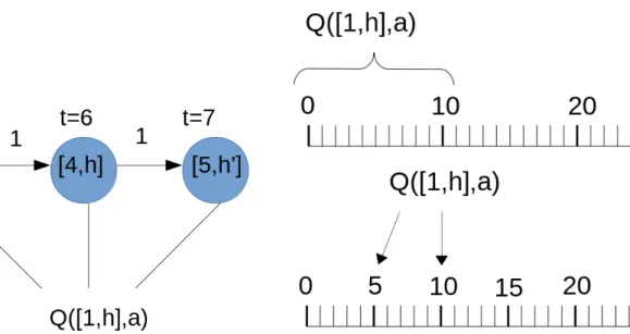
After solving the MDP at the abstract spaceStateL, an estimate of the delay delayi determined by the agent is available. We use this estimate to constrain the agent's options DiL+1 considered at the next level of abstraction: the set of options adopted by Ai in the following StateL+1 space lies in DiL+1 = {max{ 0, delayi − dL+1 }, .., delayi}, where dL+1 is the number of time instants that we subtract from the delay estimate delay to give the agent more options to consider when solving the problem in state spaceStateL+1. a) Example of local state transitions and the corresponding updated Q-value of the unitary time step, limit state space. As described in subsection 6.2.2, we take advantage of the delay estimate decided at the abstractStateLspace and effectively limit the state spaceStateL+1: After solving the MDP at the abstract spaceStateL, an estimate of the delay delayi determined by the agent is available .

We use this estimate to constrain the options of the agent DL+1i that are considered at the following level of abstraction: The set of options assumed by Ai in the nextStateL+1 space is inDiL+1 ={max{0 , delayi− dL+1}, .., delayi}, where dL+1 is the number of time instants that we subtract from the delay estimatedelayito to give the agent more options to consider when solving the problem in state spaceStateL+1. a) Example of local state transitions and the corresponding updated Q-values ​​of the Unitary Timestep, Concurrently Update Levels, Limit State Space (UTCULSS) method at. As described in subsection 6.2.2, we take advantage of the delay estimate decided at the abstractStateLspace and effectively constrain the state space StateL+1: After solving the MDP at the abstract spaceStateL, an estimate of the delay delay determined by the agent is available . Then the pure exploitation phase begins until the end of the episodes for the operational level.

Methods’ configuration

Descending Timesteps (DT)

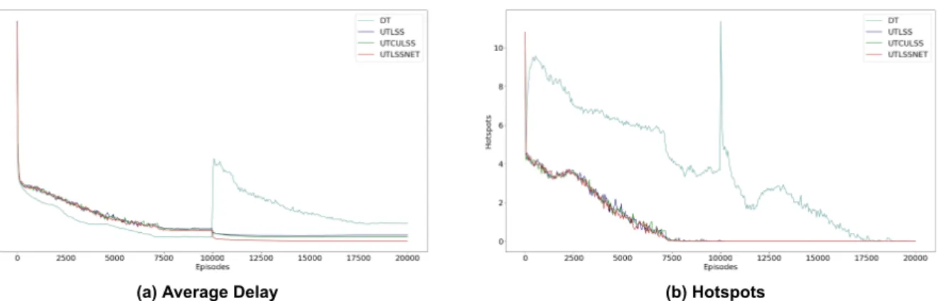
As algorithms converge to solutions, the number of hotspots should be reduced and eventually reach zero, indicating the computation of a solution, while the average delay should be reduced. Thus, the speed of reaching that point (zero hotspots) and the round at which methods stabilize agents' joint policy (which remains to zero hotspots and to a specific value for flights' average delay - without oscillating between non-solutions and /or solutions, and/or different average delay values) indicate the computational efficiency of the method in reaching solutions. It should be noted that, if a method cannot achieve a solution for a specific case, it may converge to a joint policy that does not solve all hotspots.

Distribution of delays to flights: To show how delays to flights are distributed, we provide histograms showing the number of flights with (a) 5-9 minutes delay, (b) 10-29 minutes delay, (c) 30-59 minutes delay etc. Of course, if it happens that MaxDelay is less than 60 min, 30 min etc, the histogram does not provide data for the corresponding slots of delays.

Other Methods

Efficiency of the methods

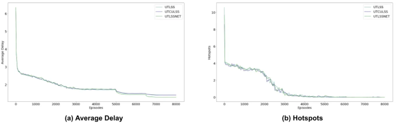
More specifically, given two levels, methods that limit the state space explored converge effectively quite early, around episode 13000, compared to the Descending Timesteps (DT) method that converges around episode 18800, as Fig. The learning curves given three levels and 10k episodes at each level, showing how agents manage to learn joint policies to solve DCB. The x-axis corresponds to the episodes, while the y-axis corresponds to the average delay per flight case (a) or the hotspots case (b).

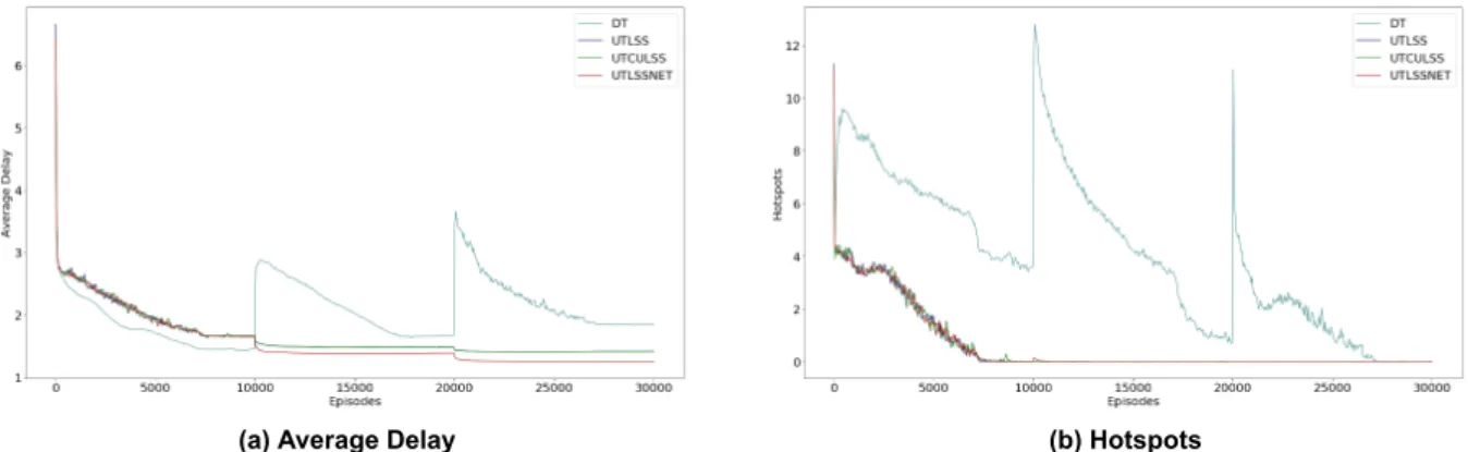
In conclusion, methods that exploit state space constraints can achieve faster convergence compared to the Descending Timesteps (DT) method. The learning curves represent three levels: 5000 episodes at level 1 and 1500 episodes at levels 2 and 3 for state space-constrained methods. Show how agents can successfully learn collective policies to solve DCB problems while reducing average delays for all flights.

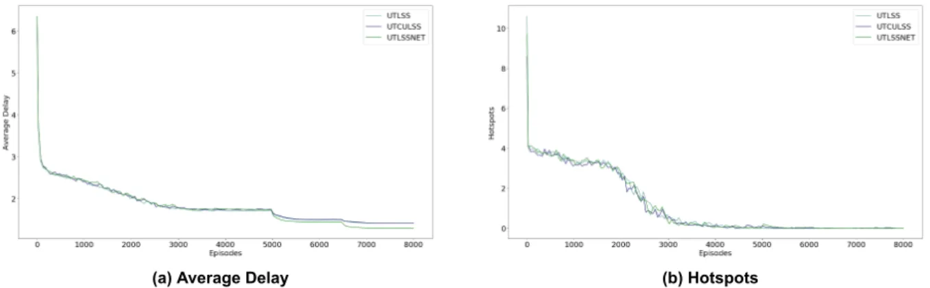
The learning curves are given at three levels, 3000 episodes at level 1 and 1500 episodes at levels 2 and 3 for methods that constrain the state space. As shown in Figure 7.4b, 3000 episodes are not enough for methods to compute solutions against zero hotspots at the first level. Even under these circumstances, the Unitary Timestep, Concurrently Update Levels, Limit State Space (UTCULSS) method and the Unitary Timestep, Limit State Space, No Experience Transfer (UTLSSNET) method manage to find a solution that results in 0 hotspots very early at the second level.

Unfortunately, this is not the case for the Unitary Timestep, Limit State Space (UTLSS) method which results in 0.2 hotspots averaged over 10 experiments.

Effectiveness of the methods to resolve imbalances

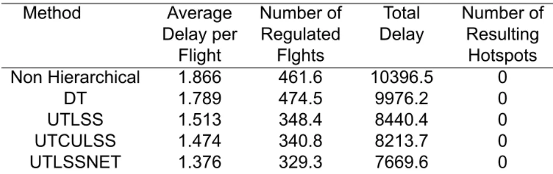
As reported in Table 7.6, all methods result in zero hotspots and hierarchical methods yield more qualitative solutions when two levels are used in terms of average delay per flight, number of scheduled flights and total delay. All other hierarchical methods manage to significantly reduce the average delay per flight, the number of flights and also the total delay when using 3 levels, compared to the results produced by 2 levels. We then present results regarding the average delay per flight, the number of scheduled flights, the total delay and the number of resulting hotspots for the cases where we significantly reduce the number of episodes.

Average delay per flight, number of regulated flights Total delay and number of resulting hotspots as reported by each method. Average delay per flight, number of regulated flights, total delay and number of resulting hotspots as reported by each method. Regarding the number of regulated flights, the methods Unitary Timestep, Limit State Space (UTLSS) and Unitary Timestep, Limit State Space, No Experience Transfer (UTLSSNET) manage to reduce them, while Unitary Timestep simultaneously updates levels, Limit State Space (UTCULSS)- the method increases them when the first level consists of 3000 episodes compared to the case where the first level consists of 5000 episodes.

All methods drastically reduce the number of regulated flights as they go from small to large delay intervals. Whereas the Unitary Timestep, Limit State Space (UTLSS) and Unitary Timestep, Concurrently Update Levels, Limit State Space (UTCULSS) methods increase the number of flights by . Whereas the Unitary Timestep, Limit State Space (UTLSS) and Unitary Timestep, Limit State Space, No Experience Transfer (UTLSSNET) methods increase the number of flights with delay in the range of 60–81 when using 3000 first-level episodes, compared to the 5000 episodes at first level.

We also investigated the effectiveness of alternative hierarchical multiagent reinforcement learning methods and alternative schemes to transfer experience between levels, to reduce delays and number of delayed flights.