This structure reveals local correlations that were not readily available in the original form of the data. In summary, the main idea of Block Hankel tensor autoregression is to extract the most important information of the time series by low-rank Tucker decomposition.
Motivation
The main idea of the discussed method is the transformation of the data to a higher order tensor via Hankelization. By doing so, we preserve the temporal continuity of the core tensors to better capture their intrinsic temporal correlations.
Thesis Outline
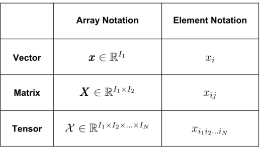
Throughout this thesis, the following notation will be used to refer to vectors, matrices, and tensors. The letter N will be used to refer to the order of a tensor and Indo to indicate the dimension of the then mode where n= 1,2, .., N.
Vectors
The in-th mode-n section of a 3rd-order tensorX ∈RI1×I2×I3 is defined as the second-order tensor (matrix) obtained by fixing the th-th mode index of X toin. The in-th mode-n plate of a tensorX ∈RI1×I2×..×IN is defined as a (N−1)-th order tensor obtained by fixing the n-th mode index of X toin.
Matrices
Trace
The outer product of two vectorsxxx∈RN, yyy∈RM is a matrix ZZZ ∈RN×M containing the product of each pair of elements of these vectors.
Matrix Rank
Matrix Products and their Properties
Tensors
- Tensor Rank
- Tensor Vectorization
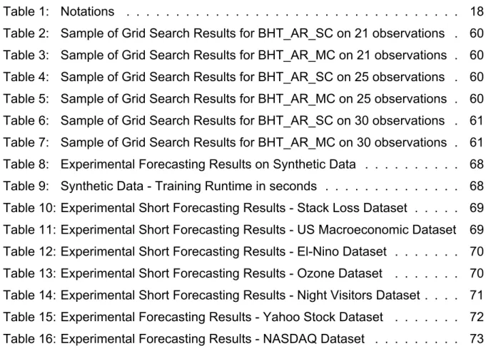
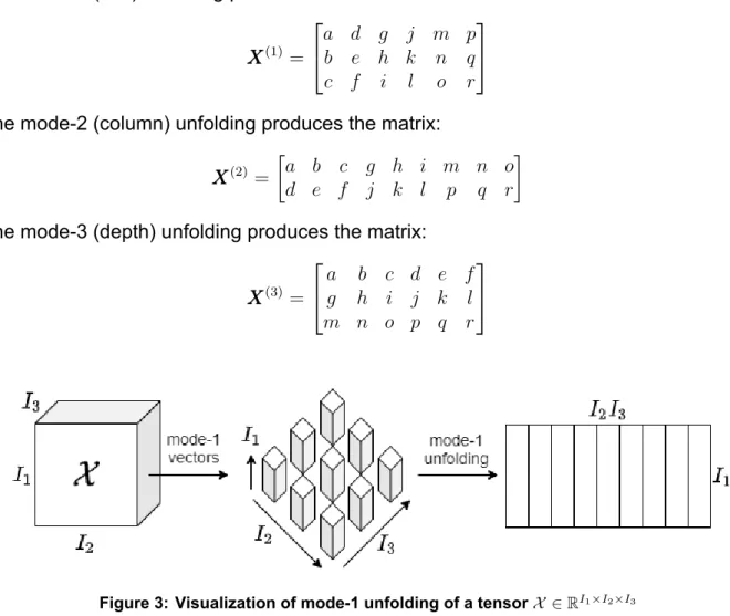
- Tensor Matricization/Unfolding
- Tensor Multiplication
- Frobenius Norm
- Tensor Decompositions
- Canonical Polyadic Decomposition
- Tucker Decomposition
Vectorization[1] is the process of converting a higher-order tensor X ∈ RI1×I2×..×IN into a vectorxxx ∈ RI1I2..IN. The Tucker decomposition[1] [4] is a model in which the tensorX ∈RI1×I2×..×IN is decomposed as a series of products of mode n between the kernel tensor G ∈RR1×R2×..×RN and a set of factor matricesUUU(n) ∈RIn×Rn.
Tensorization
Hankelization
When Hankelization of order K is applied to a vector vvv ∈ RN, it is transformed into a tensor V ∈ RI1×I2×..×IK where N. When applying Hankelization to a matrix, we must specify the mode (or modes) in which to to be implemented. Hankelization of order AK applied in the first mode would transform a matrixVVV ∈RIstart×Jinto a tensorV ∈RI1×I2×..×IK×J.
Note that when applying Hankelization in both modes, the K order may be different for each mode.
Delay Embedding Transform
- Standard Delay Embedding Transform
- Multi-way Delay Embedding Transform
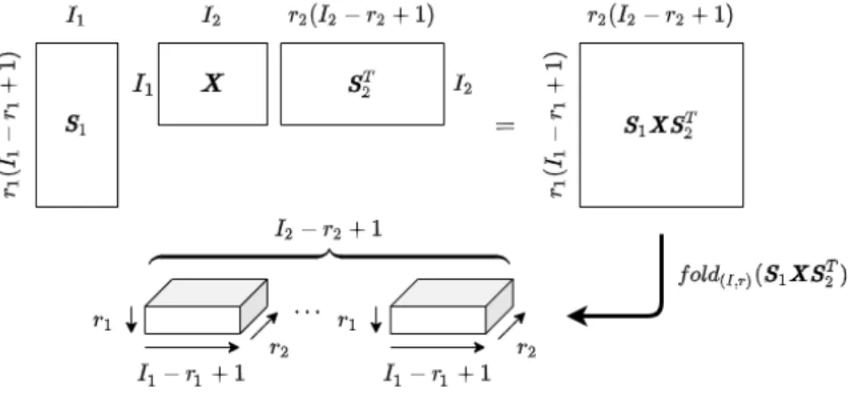
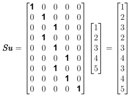
As the last step of Hankelization was the convolution operation, the first step of De-Hankelization is the vectorization of the matrix, resulting in SuSuSu. The Multi-way Delay Embedding Transform (MDT) constitutes the generalization of the Standard Delay Embedding Transform. The following figure visualizes the procedure for Multi-way Delay Embedding Transform on a matrix.
Each observation of the Block Hankel tensor is essentially a subwindow on the original data containing different timestamps. This structure can help capture the temporal correlations of the data in a more effective way. In the following paragraphs, we review each of the algorithm's components in detail and provide the necessary proofs.
In the first part of the algorithm, we use MDT to transform the data into a higher-order tensor. Therefore, this property allows us to efficiently exploit the low-rank Tucker decomposition to extract the intrinsic local correlations of the data while "compressing" the tensor. Finally, each Hankel tensor time panel is a window containing successive observations of the original time series.
Block Hankel Tensor Autoregression with Scalar Coefficients
- Updating the core tensors
- Updating the factor matrices
- Estimating the scalar coefficients
- Forecasting
Furthermore, to minimize the noise produced by the inverse decomposition procedure, we add the following term corresponding to the inverse decomposition error. To facilitate the differentiation of the above optimization problem, it is written as a sum of N terms, each of them corresponding to an n-mode unfolding. To calculate the partial derivative of (3.8) both rates above are expressed as traces.
Shang, Lie and Cheng in 2014 [9] have shown that the minimization of the set above with respect to the factor matrices UUUb(n) implies equivalent to the Procrustes orthogonality problem. The coefficients of the AR model are estimated on the kernel tensors, generalizing a Least Squares modified Yule-Walker method that supports data in the form of tensors. We estimate the coefficients by solving the following linear system, known as the Yule-Walker equations.
The prediction is concatenated with the rest of the observations along the temporal mode, resulting in the tensor Gbnew ∈ RR1×R2×..×RN×(T+1). After obtaining Gbnew, the inverse Tucker decomposition is applied using the estimated factor matrices UUUb(n) ∈ RIn×Rn, to map the data back into the original space. The algorithm requires as input the time series Xstart ∈ RJ1×..×JM×Tstart, the AR order p, the maximum number of iterations max_iter, the MDT order and the tolerance for the stopping criterion tol.
Block Hankel Tensor Autoregression with Matrix Coefficients
- Vector Autoregression with Matrix Coefficients
- Model Transformation
- Updating the core tensors
- Updating the factor matrices
- Estimating the Matrix Coefficients
- Forecasting
- The Algorithm
In this section, the goal is to derive a variation of the algorithm that overcomes the limitations imposed by the scalar coefficient autoregressive process. This subsection is devoted to autoregression with matrix coefficients to provide a better understanding of the differences between those two autoregressive processes. Therefore, given a vectorxxx, each element is written as a linear combination of the elements at the same index i, on the previous p vectors, plus a white noise quantity.
As we can see, matrix coefficient autoregression expresses each element of a vector-valued time series at a point in time, as a combination of each element of the previous observations, regardless of index, plus the intercept and white noise. Since vectorizations of different unfoldings are not always equal, we have to rearrange the elements of the first mode unfolding to obtain the vectorized form of the second mode unfolding. The prediction is concatenated with the rest of the core tensors along the temporal mode, resulting in the tensor Gbnew ∈RR1×R2×..×RN×(T+1).
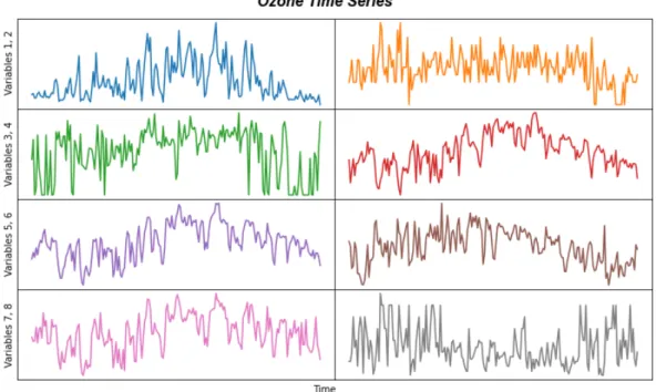
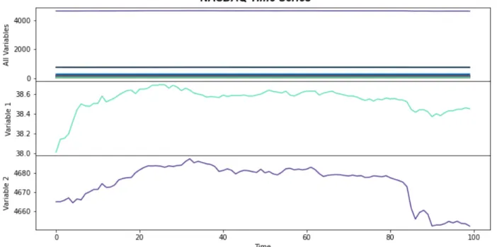
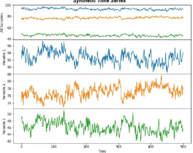
By doing so, we discard the initialization part of the generated data, which will not be representative of the time series. Thus, predicting one step into the future is equivalent to predicting the sea surface temperature for each month of the next year. The NASDAQ database contains data on 82 of the largest domestic and international non-financial securities based on market capitalization listed on the exchange [7].
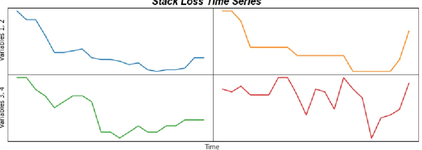
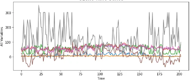
The Yahoo dataset contains 2469 observations of the daily Yahoo stock which provides information about the following variables. Note that in the case of the Block Hankel Tensor Autoregression variations, we are interested in the stationarity of the data's traded form.
Compared Algorithms
For each data set we ensure stationarity using the Augmented Dickey-Fuller test at a significance level of 5%. The Augmented Dickey-Fuller test indicates that there is insufficient statistical evidence to ensure robustness for the 7 public data sets in their original forms. The differentiation parameter will be included in the grid search that will be performed for each algorithm.
Experiments
Parameter & Convergence Analysis
In each case, the first 20 observations are used as the training set and the remaining observations serve as the validation set. Each table contains the parameter sets that resulted in the lowest NRMSE value for each validation. The row in bold contains the parameter set that produces the lowest NRMSE in the validation set.
The first 5 samples contain training sets of 20 observations and validation sets and 9 observations respectively. The remaining 4 samples contain training sets of 150 observations and validation sets of 1, 5, 10 and 15 respectively. In only a few iterations, the amount of convergence reaches and maintains a small value indicating that the changes of the UUU factor matrices are too small for the remaining iterations.
It should be noted that in all cases the convergence value of BHT_AR_MC stabilizes at a value close to zero and as a result the changes of the UUU factor matrices are invisible. Furthermore, we can see that in most cases, the NRMSE of BHT_AR_MC decreases smoothly and stabilizes near a very small value. On the other hand, the NRMSE of BHT_AR_SC shows a relatively less stable behavior.

Experiments on Forecasting Horizon
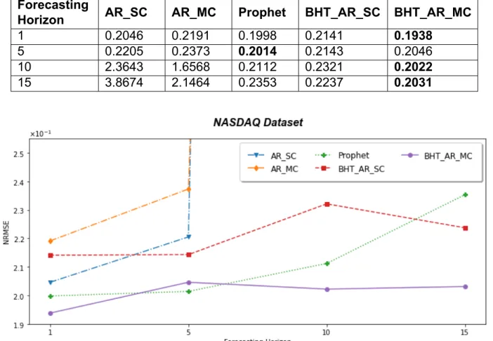
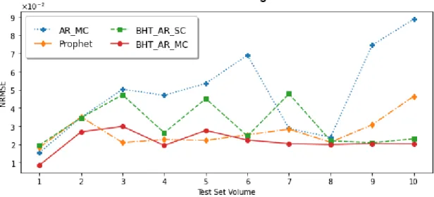
As we can see, Block Hankel Tensor Autoregression with matrix coefficients outperforms the rest of the algorithms in most cases. Moreover, it manages to maintain a stable performance in the context of short time series, regardless of the forecast horizon. Finally, although the training time for the Block Hankel Tensor Autoregression algorithms is higher compared to the traditional autoregression algorithms, it is lower than Prophet's training time.
Thus, the proposed algorithms manage to achieve excellent results while maintaining low levels of duration, which makes them an efficient and competitive choice in the context of short time series forecasting.
Short-term Forecasting Experiments
As we can see in the figures, both BHT_AR_SC and BHT_AR_MC show stability with respect to NRMSE as the volume of training data is reduced. BHT_AR_MC manages to maintain more stable performance, with smaller increases in prediction errors as the .

Long-term Forecasting experiments
Another challenge that was addressed in the long-range forecasting environment was efficiently updating the forecast as new data came in throughout the day. At each iteration a new estimate of the kernel tensors is produced, which then serves as their initialization in the next iteration. For core tensors, an incremental ranking strategy is followed in which the elements of the cores, whose rank will increase, take new random values.
The matrixization of the estimated tensor VVVˆˆˆH(θ) := ˆVVVˆˆH over the nth mode can be written as VˆH(n) =GGG(n)(2). Finally, in an effort to provide a first step towards the generalization of the algorithm, we replace the scalar coefficients of the prediction model with matrices. We performed an analysis of the convergence of algorithms and their sensitivity to user-defined hyperparameters.
However, applying Hankelization to each mode can lead to tensors of very high orders that can affect the performance of the algorithm. Therefore, we must proceed by monitoring the trade-off between the benefits of Hankelization and the performance of the algorithm. In a variation of the algorithm, we can use Tensor Train Decomposition to obtain a set of interconnected kernel tensors.