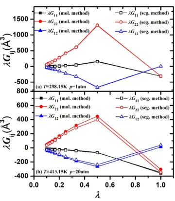
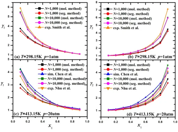
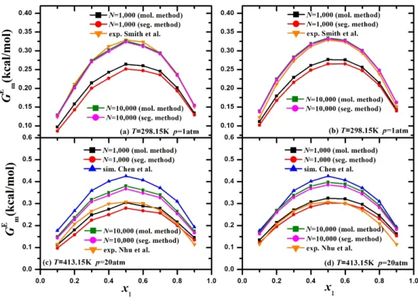
47 Figure 8: KB integrals calculated from both pair distribution functions and particle fluctuations, for n-hexane/ethanol binary mixtures with n-hexane mole fractions equal to x at T=413.15 K, p=20 atm. 49 Figure 9: Activity coefficients 1,2 plotted versus n-hexane mole fraction, x1, for n-hexane/ethanol binary mixtures, as calculated from molecule- and segment-based methods, compared to experimental data at T=298.15 K, p=1 atm 11 (a), (b). 51 Figure 10: Molar excess Gibbs energy plotted versus n-hexane mole fraction, x1, for n-hexane/ethanol binary mixtures, as calculated from molecule- and segment-based methods, using the activity coefficient method (a) and the iterative shooting method ( b).
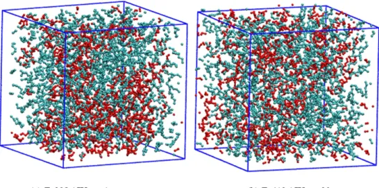
In this work, we perform molecular dynamics simulations of n-hexane/ethanol binary mixtures in the liquid state under two conditions of pressure, temperature and at different mole fractions. we first calculate the Kirkwood-Buff (KB) integrals in the isothermal-isobaric ensemble, NpT, identifying how the size of the system affects their accurate estimation of KB.
Thermodynamics of Mixing
- Kirkwood-Buff Theory
- Mixing properties
- Perfect gases
- Ideal solutions
- Real mixtures
- Gibbs energy, enthalpy and entropy of mixing
- Excess properties
In the selected µVT view, at a given time point, volume V contains exactly Ν1, Ν2, .., Νν molecules of the ν molecular species constituting the multicomponent system. In the distribution of equation (1.8), the large partition function =exp[/(kBT)] plays the role of a normalizing constant. In an ideal solution, there are interactions between molecules of component 1 and component 2, although the average energy of 1-2 interactions is equal to the average energy of 1-1 and 2-2 interactions in the corresponding pure liquids at the same temperature and pressure .
At low pressures, the fugacity fiV of component i in the vapor phase at a given pressure and temperature is proportional to the mole fraction yi, which means. Exactly the same relationship can be assumed for the liquid phase where fiL is assumed to be proportional to the liquid mole fraction xi as described in the following relationship. To replace the standard chemical potential i0, we use Eq. 1.20) for a system that forms an ideal gas mixture in the vapor phase and an ideal solution in the liquid phase, and the gas equation is subtracted from the liquid equation.
An ideal liquid solution is one in which, under constant temperature and pressure, the activity for each component is proportional to the mole fraction. When xi is close to 1, Lewis' rule applies and Ri is the fugacity of pure liquid i under the temperature and pressure of the mixture. If the relation fiL x fi i0 is respected for all components and for all compounds with fi0 being the fugacity of pure liquid i at the temperature and pressure of the mixture, then the solution is an ideal solution, obeying Lewis's law.
In this way we identify the thermodynamic consequences of molecules of one kind randomly mixing with molecules of the second kind. In ideal solutions, there are interactions between molecules, but the average energy of 1-2 interactions in the mixture is the same as the average energy of 1-1, 2-2 interactions in the pure liquids. A redundant function is the difference between the observed thermodynamic function of mixing in the real solution and the corresponding function for an ideal solution of the same pressure, temperature and composition.
Atomistic simulations
Introduction
Although many thermodynamic properties can be easily extracted (density, enthalpy), molecular simulations do not provide a standard way to estimate "statistical" properties such as entropy, chemical potential, or Gibbs energy of mixing. Over the years, various methodologies have been created and implemented to obtain such essential quantities. Widom based the extraction of all statistical thermodynamic properties on the insertion of a test particle that does not participate in the development of the system.
Following this method's basic principles, certain particle elimination methods have also been proposed.5,6 Unfortunately, methods based on particle insertion and deletion are not readily applicable to mixtures consisting of complex molecules, such as those studied in this thesis. not. KB theory not only suffers from the mentioned limitations, but also provides an effective way to calculate properties such as the Gibbs energy of mixing.
Molecular Dynamics algorithm
This corresponds to Legendre transformations from the original microcanonical to canonical (NVT) or isothermal-isobaric (NpT) ensemble. This algorithm uses the positions, velocities and accelerations at time ,t and the positions from the previous step, . All Verlet algorithms have the advantage of providing an accuracy of Ο(δt4) in positions and O(δt2) in velocities and preserve time-reversal symmetry.
Computer Clusters
Systems studied
Simulation details
The Ewald summation for Coulomb interactions has been replaced by the Particle-Particle-Mesh Method (PPPM), as we found good agreement between them and the processing time was significantly lower for PPPM. Analytical tail corrections to the Lennard-Jones interactions were applied based on the assumption of a uniform distribution of pairs beyond the cutoff radius. 1, can occur when unfavorable interactions between n-hexane and ethanol increase the vapor pressure of the mixture well above the ideal value.
Pressure composition diagrams for n-hexane/ethanol binary mixtures at T=298.15 K based on experimental data11 (top) and for T=413.15 K based on simulation results9 and experimental data10 (bottom). Deviations from ideality are not always strong enough to lead to a maximum or minimum in the phase diagram, but when they are, the consequences for distillation are significant. At the pressure and temperature at which the maximum is observed, the vapor and liquid phases, which are in equilibrium with each other, have the same composition.
Once the azeotropic composition is reached, distillation cannot separate the two components because the condensate has the same composition as the azeotropic liquid.
Force Field
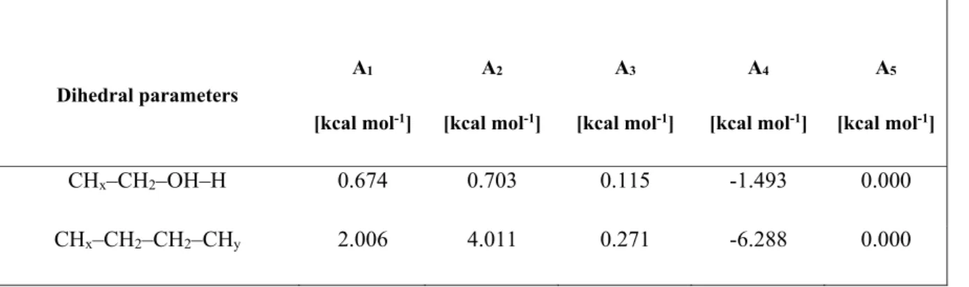
Another non-bonding interaction is the Coulomb potential, which governs interactions between atomic charges and is most commonly expressed as We also have three types of connected interactions between united atoms (pseudo-atoms) Vbonded Vbond( )l Vbend( ) Vtorsion( ) (3.5). Finally, the spin potential is very important when it comes to distinguishing trans from gauche configurations.
This potential depends on the dihedral angle formed by four consecutive atoms along a molecular chain, or, equivalently, by three consecutive bonds. This is the dihedral angle between the plane defined by the first and second bonds and the plane defined by the second and third bonds. This torsion angle potential is in the multiharmonic style of Optimized Potentials for Liquid Simulations (OPLS).
Methodology
Extension to Isobaric-Isothermal Ensemble
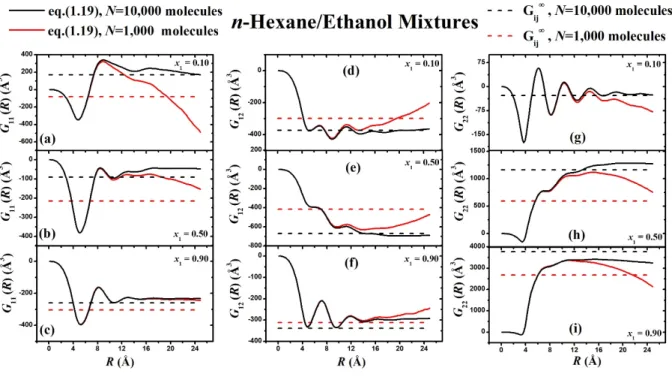
To calculate KB integrals in the thermodynamic limit from small size MD simulations, we used the recently published work by Cortes-Huerto et al. 13 They firstly introduced corrections for the extension of the μVT ensemble, where KB theory was originally developed, to the NpT ensemble and secondly for periodic boundary conditions of a finite model system such as this. They finally extracted the following expression, which connects Gij( ) KB integrals with Gij, which is the limiting value of Gij at V.
Molecule and segment based methods
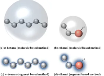
4 (c), (d) in this work, each n-hexane molecule is considered as a set of six segments centered on the centers of its skeletal combined atoms, and in the whole, each ethanol molecule is considered as three segments centered on its methyl group, its methylene group and its oxygen atom. 4 (c, d)], the greater the proportion of its molecule that it represents, and the greater the contribution to the oscillations from this segment. This behavior is similar to that observed in the works of Cortes-Huerto13 and Galata et al.
14 In this linear regime we can fit a line whose slope, according to equation (5), is Gij.
Results and Discussion
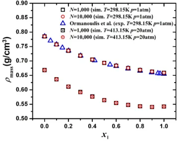
- Density
- Pair distribution functions
- Kirkwood-Buff integrals
- Activity Coefficients
- Excess Gibbs Energy, excess enthalpy, and excess entropy
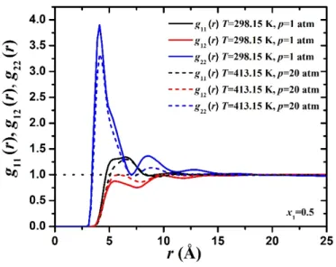
The presence of a third peak in the system T = 298.15 K, p = 1 atm indicates that ethanol tends to form chains of molecules with a hydrogen bond to the third neighbor, which is not observed at T = 413.15 K, p = 20 atm. KB integrals calculated from pair and particle fluctuation distribution functions (calculated by a molecule-based method) for n-hexane/ethanol binary mixtures with mole fractions of n-hexane x at T=413.15 K, p=20 atm. Activity coefficients 1,2 plotted against n-hexane mole fraction x1 for binary n-hexane/ethanol mixtures as calculated from molecule- and segment-based methods are compared with experimental data at T=298, 15 K, p=1 atm from Smith et al.11 (a), (b).
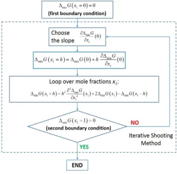
Activity coefficients 1 ,2 as calculated from molecule-based and segment-based methods compared with values extracted from Chen's9 simulations using the same force field and with experimental data from Nhu et al.10 at T=413.15 K, p=20 atm (c), (d). 9 we plot the molar excess Gibbs energy GmE N GA E versus the n-hexane mole fraction x1, as derived using activity coefficients and the iterative shooting method for both sets of systems, at T=298.15 K, p=1 atm, and at T=413.15 K, p=20 atm. Molar excess Gibbs energy is also plotted for T=413.15 K at p=20 atm, as calculated using (c) the activity coefficient method and (d) the iterative shooting method.
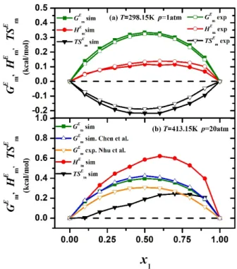
Excess molar Gibbs energy, excess molar enthalpy and excess molar entropy plotted against mole fraction of n-hexane x1 for binary mixtures of n-hexane/ethanol and compared to experimental data at T=298.15 K, p=1 atm 11 (above) . Excess molar Gibbs energy, excess molar enthalpy and excess molar entropy plotted against x1 and compared with simulation 9 by Chen et al (results extracted from the p(x1,y1) phase diagram generated in this work) and with experimental data at T =413 ,15 K, p=20 atm 10 (bottom). On the contrary, it is easily observed that HmE increases very significantly at T = 413.15 K, p = 20 atm, causing the excess molar entropy of SmE (and consequently TSmE) to change to positive quantities.
At low temperatures [T=298.15 K, p=1 atm system], where hydrogen bonding is strong, the second mechanism described above (local composition effects due to hydrogen bonding) wins and the excess entropy is negative (Figure 11, top). Thus, at T = 413.15 K, p = 20 atm, hydrogen bonding in the mixture is weak and the second mechanism described above (size difference leading to non-random mixing) wins, leading to a positive excess entropy. Unfortunately, experimental data on enthalpy of mixing are not available in the literature at T = 413.15 K and p = 20 atm to test this simulation prediction, although excess Gibbs energies are available through activity coefficient measurements.
A critique of some recent proposals for correcting the Kirkwood-Buff integrals, J. 3) Ben Naim A.; Inversion of the Kirkwood-Buff theory of solutions: Application to the water-ethanol system, J. 5) Boulougouris G.C.; Calculating the Chemical Potential Beyond the First-Order Free Energy Perturbation: From Deletion to Reinsertion, J. 6) Boulougouris G.C.; Economou I.G.; Theodorou D.N.;.