A thesis presented for the degree of Master of Science

This project is an analysis of the approach to foliations in terms of Lie∞-algebroids. We introduce the notion of holonomy, which plays a central role in the study of the local foliation structure around a given leaf.

Definitions and first examples

As in the previous case, the covering projection D×R→D×S1 induces a foliation on the solid torus D¯×S1, which is called the Reeb foliation. The stratification of F from M codimensionq can be described as. i) the maximal foiled atlas {(Ui, φi)}, (ii) the Haefliger wheel of codimension q, (iii) the smooth involutive subsheaf T M.

Constructions

If necessary, we can make a refinement of this atlas so that the coefficient constraint mapq:M →M/Gto everyUi is injective. Although this is actually a special case of coefficient foliation, it is usually discussed separately.

Holonomy

We say that the holonomy is invariant of the choice of cross sections in the above sense. Its image, called the holonomic group of Latx, is denoted by HolT ,T(L, x) and by property 3 above, is unique up to conjugation in the following sense: ifT, T0 are cross sections at x, then HolT ,T ( L, x) andHolT0,T0(L, x) are conjugate subgroups of Diff0(Rq).

Foliations and Lie groupoids

Lie groupoids in differential geometry

A basic groupoid M is a groupoid over M whose set of arrows consists of homotopy classes of paths in M. We define the gauge groupoid Gauge(P) connected to P as a groupoid over M whose morphisms are the orbits of the diagonal action ofGin P×P, i.e.

The monodromy and holonomy groupoid of a foliated manifold

The leaves of the foliation M induced by the Lie algebroid(T∗M,[·,·]T∗M, π]) are symplectic manifolds (see [34]). For every almost Lie algebroid(A,{·,·}, ρ), the image of the anchor chart is a singular foliation on M.

Under the microscope: Geometric Resolutions

• A pinch of homological algebra
• Existence of geometric resolutions
• Resolutions in the smooth category
• Examples

A real analytic geometric resolution of a singular real analytic leafF is also a smooth geometric resolution of the smooth leaf generated by F. Every finitely generated algebraic geometric resolution of an open Zarisky subgroup of Cn admits a geometric resolution of length at most n+1 Now, suppose that (E, d, ρ) is a geometric resolution for F, which means that we have an exact sequence of bundles.

We want to prove that (E, d, ρ) is a smooth geometric solution of the smooth foliation F∞, and therefore we need to check the accuracy of the sequence. In the next step we continue with the component -n+1 and by iterating this process we obtain a geometric solution of length n and with trivial vector bundle at degreei≥2. A locally real-analytic smooth singular foliation of a smooth manifoldM allows a geometric resolution of length at most dimM+ 1 over any relatively compact open subgroup ofM.

We will prove a stronger claim: any locally real-analytic foliation admits a finite-length geometric resolution over any relatively compact open subset of the manifold. Similarly, one has a geometric resolution of length 1 across the foliation defined by the action of so2onR2.

Graded Manifolds

Vector fields

The most natural way to describe vector fields in the graded-geometric world is by thinking about their derivative property. A vector field X oneE of degree k is a graded derivative of the bundle of functionsE of degree k, i.e. We say that a vector field has arityk if it maps functions of arityk to functions of arityk+l.

Moreover, a function of arity 2 would be an element in Γ(E∗)Γ(E∗) and so from the derivation property ofX it follows that. We can now describe the local shapes of vector fields in terms of partial derivatives. It follows that the local sectionsXU ∈ ΓU(E) coincide on the overlapU ∩V of open coordinate domains and therefore they define a global sectionX ∈Γ(E) such thatX|U =XU.

Let E = (E−i)i≥1 be a graded manifold with bundle of functions E and denote by E˜ the Euler vector field onE, given by3.10. It is therefore sufficient to prove the first part of the Lemma, for a vector field X of degree and artyr.

Duality of higher structures

L ∞ algebras and Lie ∞-algebroids

Moreover, this is a derivation of degree +1 from the graded Lie bracket: for each homogeneous element x, y. We want to weaken the Jacobi identity condition satisfied by the bracket [·,·] :=l2 and impose that it is only satisfied up to homotopy in the sense that there exists a skew-symmetric mapl3:V3. The component E−1 of a Lie ∞-algebroidE overM has a near-Lie algebroid structure and induces a foliation of M.

Moreover, the constraint{·,·}|Γ(E−1) satisfies the Leibnitz rule by definition, and furthermore the anchor mappingρ:E−1 →M of the Lie∞-algebroid preserves the 2-bracket. There is a one-to-one correspondence between Lie algebraic structures on the vector bundle A→M and Lie 1-algebroid structures on A[1]. In general, the algebraic structure of a Lie∞-algebroid can be significantly more complicated than that of a Lie algebroid.

There is a one-to-one correspondence between Lie algebraic structures on a vector group A→M and Q-manifold structures on A[1]. Given a vector bundleA→M, we first describe how a Lie algebraic structure onA defines a homologous vector field in A[1].

Q-manifolds and Lie ∞-algebroids

Assume that ∆ ∈ Lis odd and denote by J∆n the Jacobiators of the higher derivative brackets of . After a few pages of calculations, thoroughly performed by Voronov in [32], we deduce that the JacobiatorsJ∆n are governed by the higher derivative brackets of ∆2. The lie bracket of vector fields respects the arity rating, which implies the following Lemma.

Recall that the arity components of the graded vector field commutator are determined by. In particular, this means that the k-brackets on Γ(E) given by 3.38 are compatible in the spirit of higher Jacobi identities. Based on the example of the Lie algebroid and expression 3.27 of the anchor chart in the sense of the action of the homologous vector field on smooth functions, we consider the morphism of the vector bundle defined by

The Leibniz property of the graded commutator, combined with the disappearance of contractions on smooth functions, indicates that f will eventually escape the bracket. Moreover, it follows from the previous statement that the differentiated: Γ(E)→Γ(E) can be seen as a set of O-linear maps d(i): Γ(E−i)→Γ(E−i+1) .

Morphisms and homotopy

At this point, we should discuss an aspect of gold components that will be useful for our work in Chapter 4. A morphism of Lie∞-algebroids (or Lie∞-morphism) from (E, QE) to (F, QF) is a morphism of the sheaf of scaled algebras, Φ :F → E, of degree 0 such that. The Gold 0 component of Φ is restricted to a chain map between linear parts of Lie∞-algebroids.

The chain mapφis called the linear part of the Lie ∞-morphism Φ. The following definition can be considered a generalization of derivations of a graded algebra. It is an operator of degree +1 which is quadratically zero, due to the homologous property of QE and QF. According to isomorphism4.1, vertical vector fields with arity n-1 and degree k can be represented as (possibly) infinite sums of elements in the antidiagonalsi−j = k(height-depth=degree) in the sections of the bicomplex.

This implies that the cohomology groups are isomorphic, so we develop our proof in the context of the bicomplex4.2. It immediately follows that these data induce a near-Lie algebroid structure on A, following an application of the decalage isomorphism3.20.

The Lie ∞-algebroid resolving a singular foliation

By Proposition 2.2, the vector set E−1 carries an almost Lie algebraoid structure with anchor map ρ. Note that such existenceY is equivalent to an extension of the quasi-Lie bracket onE−1 in Γ(E). We have the decomposition of R2 into these leaves: the origin, the connected x-axis components without the origin, and lines parallel to the x-axis.

We will construct a Lie∞-algebroid structure (a Lie 2-algebroid structure, more precisely) onE= (E−i)i=1,2 in the form of parentheses. Recall that the compatibility relation between the differential and the 2-bracket of a Lie ∞-algebroid is given by the higher Jacobi identity for n=2. By an iteration of this method, we get the rest of the brackets between the generators of Γ(E−1) and Γ(E−2).

Recall that the brackets of a Lien algebroid vanish for k≥n+ 2, so in this example, there are only 3-brackets left to define. Since the latter operator is injective, we conclude that a 3-bracket in Γ(E) that is compatible with the differential d and the 2{·,·} bracket must be zero everywhere.

The universality of a Lie ∞-algebroid resolving a foliation

Φ-derivations

Let (E, QE) and (F, QF) be Lie∞-algebroids over M and let Φ :E → F be an O-linear morphism of graded algebras. Denote the space of O-linear derivatives Φ of arytynnga D(n) and consider the operator∂ onD(n) given by. 4.23) After some direct calculations, identical to those in the proof of Proposition 3.8, we arrive at the following Lemma. If δ is an O-linear derivative Φ of n degree k+ 1, then∂(δ) is an O-linear derivative Φ of n degree k+ 1.

Any O-linear Φ-derivationδ of arytyne can be restricted to an O-linear map ˆδ: Γ(E∗)→Γ(Sn+1F∗) and it can therefore be identified with a section in Γ(Sn+1F∗⊗E ). Conceptually, such a derivationδ of arytyn and degreek, can be written in local coordinates (ξa),(ξb) for F∗ and E respectively, which. A Φ derivative of arytyn and degreek can be represented as a sum of elements in the antidiagonals i−j =k (height-depth=degree) in the sections of the bicomplex.

Note first that the lines in the bicomplex 4.24 are exact at the level of sections, except perhaps at depth 1. Such an element can be represented in the bicomplex 4.26 by an anti-diagonal lying in a sub-bicomplex with exact lines at each position.

The survey towards universality

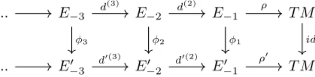
Any chain map φ:F →E between the linear parts of the two algebroids is the linear part of a Lie∞-morphism from (F, QF) to (E, QE). It is indeed the case that two Lie∞ morphisms with the same linear part are homotopic. In particular, this implies that (Φt)t∈[0,1] is a differentiable path for Lie ∞ morphisms, and that χ = ​​Φt=1 is also a Lie ∞ morphism.

A homotopy deformation of ΦtoΨto arytyne is a sequence of Lie∞-morphisms(Φk)−1≤k≤n such that. ii). Let ΦandΨbe Lie∞-morphisms such that there exists a homotopy deformation of ΦtoΨof arity. Let ΦandΨ be two Lie ∞-morphisms such that there exists a homotopy deformation of arity +∞from ΦtoΨ.

Then any two Lie∞-morphismsΦ,Ψfrom(F, QF)to(E, QE) whose respective linear parts φandψ are homopic. By Proposition4.4Φt=1 and Ψ are homotopic Lie∞ morphisms and by the transitive property of homotopy between Lie∞ morphisms, it follows that Φ is homotopic to Ψ.