A transformation like that of Einstein and Rosen does not limit the geometry of spacetime. The shaded regions present the singularities at the center of the black hole and the white hole.
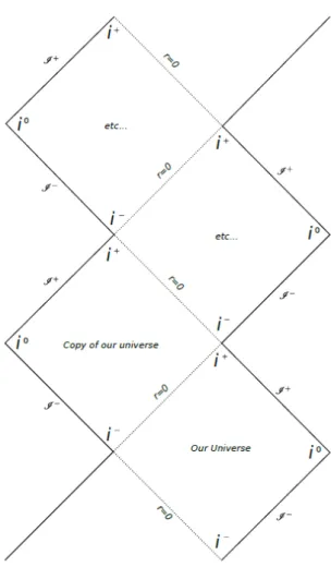
![Figure 1.1: The regions of the Kruskal diagram.(This graph has been taken from [3]) IV are in someway unexpected](https://thumb-eu.123doks.com/thumbv2/pdfplayerco/333518.53533/10.892.364.531.281.448/figure-regions-kruskal-diagram-graph-taken-someway-unexpected.webp)
The metric should be static and spherically symmetric
As we know, the regularity of spacetime is verified by the scalar invariants produced by the Riemann tensor. Scalar invariants are produced by contractions of the Riemann tensor or the Ricci tensor.
For a wormhole solution, there must be a throat connecting two spacetime
This minimum value is the throat of the worm, which we will examine below. As we said before, the throat is the minimum of the function r = r(u), which is taken at u = 0.

For a traversable wormhole, no horizon should be present
In this way, Vishveshwara concludes that the two basic properties of Schwarzschild's event horizon are satisfied by the null hypersurfaces, defined by KμKμ = 0 (killing horizon), for a general spherically symmetric and static metric. In other words, if a particle or photon crosses the event horizon from the region of spacetime associated with infinity, it is impossible to return to the outside from which it came.
The wormhole metric has to satisfy Einstein’s field equations (The Stress
Substituting the Ricci tensor Rµν = Rρµρν and using the antisymmetry of the Riemann tensor for Rσµ. In wormhole physics, we mainly deal with NEC, since its violation in the throat is a characteristic feature.
Morris and Thorne metric
The shape of the wormhole is determined by the specification of the ratio between r and l. In section [2.2] we proved that in the case of α= 0 the burnout condition is guaranteed by the constraints of the r = r(u) function. In the previous chapter, we expressed the Stress-Energy tensor components in terms of the α, β, γ functions of the metric (2.1).
Thus, since there is no restriction on the sign of b′(r0), there is no restriction on the sign of the energy density. We can therefore apply the Lorentz boost to the mixed components of the Stress-Energy tensor. Thus, (2.70) is satisfied, while in the light of (2.74) we see that in this case the energy density is negative at the throat, even for the static observer standing there.
The causal structure of a traversable wormhole
We can either state some specific conditions for the center of space to be regular or we can construct a centerless spacetime, i.e. The second way is already known from the construction of wormholes that we studied earlier. As shown in the paper by Simpson and Visser, the metric adjustment implies NEC violation in all time space except possible horizons.
From there we can see the metric (3.2) as a combination of the initial-input metric and the trivial wormhole example of Morris and Thorne. Although on top of that we also need to avoid any event horizon for the new metric. But we prove that in the case of the Gaussian coordinates, for which we have a vanishing α of the general metric (2.1).

From Schwarzschild black hole to traversable wormhole
Introducing a negative cosmological constant
The components of the Riemann tensor are similar to (3.28), but with an additional term, which indicates the existence of the cosmological constant. Kretschmann's scalar is huge, ugly, and for these reasons useless to write down. The first is the Kretschmann scalar in the case of a cosmological constant of zero, the second is proportional to |Λ|, while the third is proportional to |Λ|2.
But it is clear even from the components of the Riemann tensor that spacetime is regular, since no component becomes infinite. If we take the limit u→ ±∞, we take R → −4|Λ|; that is, a constant negative scalar curvature which corresponds to an AdS spacetime.
Introducing a positive cosmological constant
As we said, just change the sign to the cosmological constant and you'll find them. For each η satisfying (3.35), a cosmological horizon is defined far from the throat where NEC1 is not violated. For these values, the event and cosmological horizon of the initial black hole are located at rh ≈2.027M and rc ≈16.217M.
In the first graph we see the behavior of ρ+p1 around the throat, which is similar to that of Figure 3.1, albeit with different values of η, adapted to the location of the initial event horizon. The behavior of ρ+p1 around the cosmological horizon is shown in the second graph, for u > 0 (the behavior for u < 0 is symmetric). At the cosmological horizon, ρ+p1 reaches zero, while outside the cosmological horizon we see that it remains negative, with a negative minimum value and then goes to zero for large values of the coordinate u.

From Reissner–Nordström black hole to traversable wormhole
Introducing a negative cosmological constant
As we see in Appendix B, the introduction of a negative cosmological constant affects the Reissner–Nordström black hole to have a metric of the form (B.7) with Λ =−|Λ|. The fading condition is met, since gtt for (B.7) is negative forr > rh. Regularity, asymptotic behavior, Stress-Energy tensor and NEC violation The contribution of the cosmological constant to the tensor components (Riemann and Stress-Energy tensor) is the same as in the case of the Schwarzschild metric.
The only difference is that the terms with index correspond to the terms with non-vanishing Q given in the previous subsection. Therefore, the regularity is guaranteed, while for the limit u → ±∞ we again take R → −4|Λ|; that is, two asymptotically AdS spacetimes. A negative cosmological constant does not introduce any cosmological horizon, so again the NEC is violated for every u.
Introducing a positive cosmological constant
For this value of Q and Λ, the event horizon of the initial black hole is located at rh ≈ 1.44M and the cosmological horizon at rc ≈ 16.24M. On the left we see ρ−p1 around the throat, while on the right we are close to the cosmological horizon.

Black-Bounce and One-way traversable wormhole
In the case of the timelike geodesics, the affine parameter can be taken as the real time (τ), while for the null geodesics only an arbitrary affine parameter remains. Our aim is to simplify the above equation as much as possible, in view of the symmetries of spacetime; that is, the spherical symmetry and the staticity of spacetime (I follow [11]. The other characteristic of the spherical symmetry is the existence of a rotation Killing vector; namely the Killing vector: R = ∂φ.
This Killing vector represents the rotational symmetry about the z-axis and as we saw in the example of chapter (2.1), the corresponding conserved quantity can be interpreted as the angular momentum of the particle (per unit rest mass). Staticity: The fact that our metric is static is reflected by the existence of the timelike Killing vector (2.10). By making use of the symmetries of spacetime, the problem has been reduced to a one-dimensional problem.
The circular orbits as a tool for distinction
Photon spheres correspond to circular orbits of null geodesics, while ISCOs correspond to stable orbits of time-like geodesics. Since photon spheres and ISCOs do not coincide, it is possible that some ISCO throat values are defined but photon spheres are not. Furthermore, it is obvious from the above consideration that as the throat becomes larger and larger, the location of the circular orbits decreases until it does not exist at all.
This can be understood as the fact that as we open the throat more and more, it becomes larger than the event horizon and then the horizon is not allowed.
Distinguishing the Schwarzschild black hole from the traversable wormhole 46
This means that if a photon sphere is allowed for the wormhole, no time-like circular orbit can be defined outside the photon sphere. But if the photon sphere is not allowed, which is for η > 3M, then there is no such restriction for a time-like circular orbit. If we compare the values of η that allow the photon sphere and the ISCO, we see that:.
4.20) Setting Q= 0 we see that the root with the minus sign goes to zero, while the root with the plus sign goes to 3M, which is the photon sphere of the Schwarzschild metric. But are we sure that the location of the photon sphere of the Reissner–Nordström black hole is larger than its event horizon. In (4.23) the denominator is the quartic equation that defines the location of the photon sphere.

Effective Potentials and particles’ behaviour
Schwarzschild case
In Figure 4.5 we present the effective potential of each case and for L2 = 14M2; that is, an angular momentum greater than that of the ISCO. Therefore, assuming large values of angular momentum, there are two circular orbits; one stable and one unstable. At the minimum value of angular momentum, these two orbits coincide and form a stable orbit at the throat and no ISCO.
In the graph above, we see the angular momentum squared with respect to the radial coordinate u. The blue regions correspond to the angular momentum values that allow only a circular orbit. Therefore, comparing the above with (4.27), we see that the angular momentum is consistent with Newtonian gravity away from the nozzle (weak field limit).

Reissner–Nordström case
For a traversable wormhole, there must be no center in the geometry; definition of the neck. The second [13] concerns an extension of the Simpson-Visser technique to Reissner-Nordström and Kerr black holes. But a wormhole geometry is achieved by requiring a neck to spacetime; a requirement that limits the gθθ component of the metric.
In Chapter 1 we saw that this last constraint is responsible for the violation of the Zero Energy Condition. The difference between the above and (1.3) is that instead of the matter Tµν in the r.h.s we have an effective energy-momentum tensor. The zero energy state, according to the modified theory, is expressed in terms of the effective energy momentum tensor, rather than in the matter field itself.
Let's see how a transition from a black bounce to a traversable wormhole can be described by this model, in the case of the incoming zero coordinate. The fact that we use the zero-ingoing coordinate w means that the energy flow is directed towards the apparent horizon (in view of "our" universe which we assume is u > 0) of the black bounce.
