This is a favorable area for Corelab, due to the work of Stahis Zachos and Aris Pagourtzis; more importantly, it proved to be a creative way to both better explore triangulation problems, plus to engage me in an area I initially thought didn't "speak". My justification lies in at least one of the following: they are simple and easy to verify their correctness;.
Motivation
Preliminaries
- Geometric graphs and (fixed) graphs’ drawings
- Intersection vs. crossing of segments
- Convex geometric graphs
- Isomorphism in the context of convex geometric graphs
- Planarity
For our convenience, we will use modulo arithmetic to refer to the indices of the vertices of a convex geometric graph, i.e. A graph is called planar if it can be drawn on the plane without crossing edges. Within the context of geometric graphs, planarity loses its strength, since we are not concerned with whether the underlying abstract graph is flat, we focus in the specific drawing on the plane (see Figure 1.2).
An abstract graph G is called extraplanar if it can be drawn on a plane without crossing edges and with all vertices in the outer region of the drawing ([8]); equivalently, no vertex is completely surrounded by edges. A long-standing result of Lloyd [26] from 1977 states that: "given a set V of points in a plane and a subset E of segments with endpoints in V, it is NP-hard to determine whether there is a triangulation of V". Also, for completeness, we prove a simple lemma that relates our triangulation to the largest set of pairwise noncrossing segments at n points in the plane.
The convex point set case
In Chapter 5 [3], we showed that for CIRCLE graphs, changing the original definition to use the term "cross graph" instead of "intersection graph" has no effect on the class itself1. We can now present a theorem relating our problem to an independent set on CIRCLE graphs. In a few words, by taking advantage of membership in the CIRCLE class, a Circle Independent Set (CIS) can be seen as finding the set of k chords of a circle that are not pairwise intersecting.
All we have to do is recall that placing the points of V around an arbitrary circle Cin the same order of appearance as inV (functionf :V →C) is sufficient to ensure that exactly every intersection of E by f preserves becomes and no new crossings. appears (see [3], Chapter 3). It takes no more time than performing a convex hull algorithm to find the order of the points of V (O(|V|logh(V)), [7]).
Polygon triangulation existence ( Poly-TRI )
A result of Wigderson (1982) states that given a maximal planar graph, it is NP-complete to determine whether it has a Hamiltonian circuit. We will consider this (Max Planar HC) as our well-known NP-complete problem and establish a polynomial-time reduction to Poly-TRI. Finally, we will need to efficiently draw any given case on the plane such that the geometric graph (V, E) has a polygonal triangle if and only if the abstract Gha has a Hamiltonian circuit.
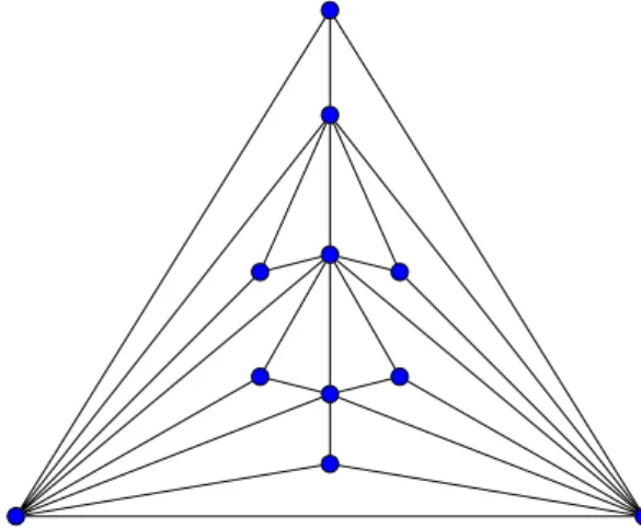
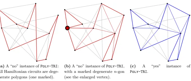
Then D(G) cannot have a polygonal triangle TP because being true will force a Hamiltonian circuit in G; contradiction. Whatever the drawing D, D(C) is a simple polygon at all points/vertices and its interior region is triangular because all faces of a maximal planar graph are triangles. An illustrated example: we can consider the Golder-Harary graph, introduced in 1975 (Figure 2.4), the smallest of the class of maximal planar graphs that do not have a Hamiltonian circuit.
Notes on triangulation existence
First, we give a few words on the basics of enumeration complexity and describe the reductions used to show the hardness results for #P. P is the class of functions that count the exact number of accepting paths of a polynomial-time nondeterministic Turing machine (PNTM). So, changing the reductions in Karp can give a better characterization of enumeration problems with the easy decision version (#PE).
In this direction, the work of Pagourtzis and Zachos [30], together with the definition of the very interesting TotP (in [23]) and the results in [23] and [24], gives a detailed overview of the structure and relations between counting complex classes. FP is a class of counting problems for which a polynomial time deterministic Turing machine (PDTM) exists. TotP is a class of functions that count the total number of computational paths of a PNTM.
Counting complexity for the convex case
We will say that a Karp reduction of A to B is weakly parsimonious if for the mapping function f there exists a polynomially computable functiong that has A #Awitnesses if and only if Bhasg(#A) is a witness. The term "weakly parsimonious" often appears in the bibliography, although there are several corresponding terms, one-to-many, many-to-one, even a very specific definition and example of bit-shifting reductions [25]. We determine whether the problem belongs to TotP by proving the correctness of Algorithm 1 and, of course, its polynomial running time.
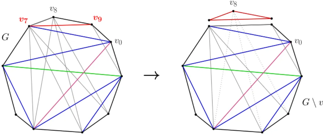
For the rest of this section, we will use the traditional graph notation by a single letter (eg G), but always assume that this graph is fixed at a convex position on R2. Let vi−1vi+1 be part of triangulations TC1, .., TCk, k ≥ 0 (note that the proof also holds for the set of triangulations that is empty). Therefore, any other edge of any TCi can be seen as an edge of the convex graph induced from G by deleting vertexvi.
Counting complexity of Poly-TRI
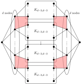
Due to the technical nature of the reduction, we abandon the sketch, as it would take up an unnecessarily large part of the thesis without offering new perspectives or better intuition. Let G be a graph that has N as an induced subgraph such that only its outer face vertices – denoted by zorw – are adjacent to edges that are not in N. a). Furthermore, we can reasonably consider the first of the two different processes of the algorithm as a preprocessing step running in O(n2) time, since multiple triangulations of convex polygons of the same size may need to be generated.
The consideration of different triangulations of a point set first appears in a well-studied form in the mid-18th century by Leonhard Euler: he successfully conjectured the closed formula for the number of triangulations of the convex n-gon, which was what we now denote Cn−2, the (n−2)th Catalan number. Another modern take on the same core problems is the efficient generation of random triangulations of point sets. An alternative way to attack triangulations is through structures and procedures that are related and move along similar structures, usually triangulations that differ from each other by a single reversal: Hurtado and Noy's work builds a tree of convex triangulations, with a parent-child relationship resolved by an edge flip; Molloy et al. and McShine and Tetali[27] build random walks on relevant structures using the same principle and study their mixing time – the latter obtaining an approximate sampling algorithm running in O(n5) time.
![Figure 3.3: Core of the reduction by Wigderson [42], based on the “gadget” subgraph N](https://thumb-eu.123doks.com/thumbv2/pdfplayerco/292642.39160/38.892.179.694.661.808/figure-core-reduction-wigderson-42-based-gadget-subgraph.webp)
Preliminaries
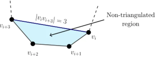
As an analogue to the notion of consecutive vertices, given an appropriate convex polygon label, we define two consecutive span-2 edges to be a pair of edges of the formvi−1vi+1,vivi+2. Every triangle of a convex geometric graph on 5 or more vertices has at least two edges of space-2. Since all n non-diagonal edges of TC are sides of n−2 triangles, by the pigeonhole principle, there are at least 2 triangles that use 2 sides of the n-gon as their sides.
A convex geometric graph with n≥5 and only two 2 span-2 edges appearing consecutively in the drawing has no triangulation. Two consecutive span-2 edges intersect, so together they do not form a triangle, unless only one is needed (quadrilateral). There must therefore be a third span-2 edge which, together with one of the 2 consecutive ones, is the obligatory second span-2 edge in a triangulation T of the graph (see Theorem 4.2).
The reduction argument and recursive relation
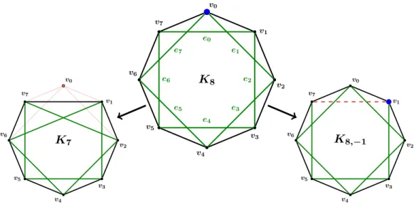
The left subtree contains all triangulations of a K7, which become all triangulations of the initial K8, including e0; while the right subtree contains all triangulations of the octagon that do not contain e0. Obviously, this applies to all branches of the tree, as they are all made in the same way. It proves that the key to our reduction is the correct definition of the next vertex (or span-2 edge) to work on.
For each new graph, keep a 1×n table to indicate the mapping from the current to the initial labeling; current missing vertices of the parent graph can be highlighted (for example −1 items). Each node denoting Kr,−m takes O(n) time to be created and coded: store the integers r and m, the 1×n mapping matrix for labeling the vertices, plus an indicator of 2 integers numbers to go back to the parent node: if it's a left child, hold [vm,−1], for a right child, hold [vm−1, vm+1], where vm is the critical vertex of the parent node relative to the situation. For each node, the triangulations encoded in the left subtree are not connected to those of the right subtree because they differ from each other at the edge.
The algorithm
Note also that even if it is not directly apparent that T1 differs from T4, our simple branching rule guarantees that T1 includes v4v1 as an edge, while T4 does not, since they belong to a different subtree of the root node that branch is w.r.t.v0/v4v1 . Therefore, it is clear that O(n) bits are sufficient to encode all triangulations of the convex gon. We get a triangulationTC from a convex-gon triangulation, and proceed almost identically as in Algorithm 2; only now the branch condition checks the edges of the polygon (see Algorithm3).
For both algorithms, it is easy to show that they branch with probability analogous to the triangulations of each of the two subtrees rooted at the two children (see Figure 4.6). A nice way to see this is using the recursive relation and Figure 4.5: starting at Tn,0, you can move 1 square to the north (left child) or 1 to the east (right child). Otherwise, you can either move to the northwest square (left child) or the east square (right child).

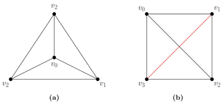
![Figure 2.2: Triangulation existence given a convex geometric graph. Due to the properties of convex graph drawings ([3]), we are allowed to show any convex point set as on a single circle without loss of generality.](https://thumb-eu.123doks.com/thumbv2/pdfplayerco/292642.39160/27.892.217.705.502.746/figure-triangulation-existence-geometric-properties-drawings-allowed-generality.webp)