[PENDING] Unsteady shear layer roll-up modeling

These instabilities lead to a chaotic behavior of the shear layer development with time. This immediately means that Geometric and Motion Preprocessor Programs will be needed to generate the geometry and motion of the wing.

Main Considerations

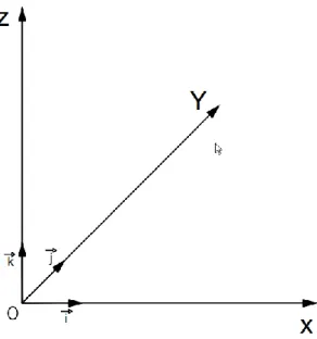
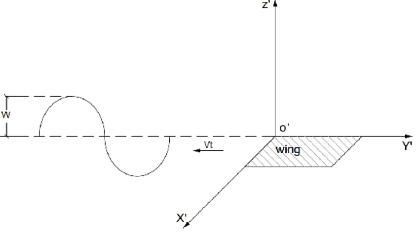
Definition of Frame of Reference

In general, the location of the relative position of 𝑂′𝑋′𝑌′𝑍′ with respect to 𝑂𝑋𝑌𝑍 can be seen in Figure 2. 𝐴 of a point A with respect to 𝑂′𝑋′𝑌′𝑍′ at a time 't ', Figure 2, and we want to find the position 𝑅⃗⃗𝐴 with respect to 𝑂𝑋𝑌𝑍.

Motion and the No-Entrance Condition

For an observer in the IFoR, the velocities acting on the body are the translational velocity and the swing velocity. As can be observed from the above equations, an observer in the 𝑂𝑋𝑌𝑍 system measures different velocities for different points on the wing.

Vortex Lattice Method (VLM)

The subscript (tr) refers to the trace of a function at a point A on the boundary and is defined as the limit of the function as it approaches the point A. The camber of an airfoil is defined as the average line from the top and bottom of the airfoil. This means that we can distinguish between an upper 𝑆𝑐+ and lower 𝑆𝑐− side of the camber surface.

The right side of the system includes the resultant velocity at each of the individual points of the body in the normal direction and the normal velocities induced by the wake at these points, without the Kutta strip. The first strip of the wake is the 'Kutta' strip and is discretized by the Kutta strip panels, while the rest of the wake is discretized by the wake panels, Figure 13. At the collocation points of the vortex panels we implement the no-entry boundary condition, while at the Kutta strip points we implement the Kutta condition.

In addition, on the common boundary of the vortex panels we define a control point, which is used for the calculation of forces and pressure. 𝐾𝐿 in equation (57) is called the induction factors from the line segment KL (belonging to the MN panel) to the collocation point of the IJ panel. At this time step, the algorithm has already calculated the 𝛤𝐼𝐽 on the body and the Kutta strip at the end of the previous time step and has already calculated the position and 𝛤𝐼𝐽 of the wake.

Describing the Method

Equations used in our modeling

Equation (63) states that as you approach the trailing edge from the suction side (top) and the pressure side (bottom), the pressures on both sides become equal. Where 𝑝+, 𝑝− is the pressure on the upper and lower part of the wake surface at the same point.

Modeling of vorticity

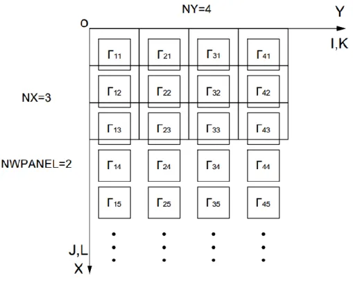
The vortex grid method is an extension of the "lumped-vortex method", in which the vortex strengths are placed at a quarter of the length of each plate in the chord direction, while the boundary conditions are satisfied at the collocation points (three quarters of the length of each plate in the chord direction) [22]. In our modeling, the indices 𝑖, 𝑗 describe the strength of the vortex (i.e. control points), while the indices 𝑘, 𝑙 describe collocation points. At this stage we need to distinguish between a geometry/body plate and a vortex plate.

The first one refers to the discretization of the wing geometry in rectilinear plates, where each geometric plate has width 𝛥𝑌𝑔 =𝑠𝑝𝑎𝑛. A Kutta-type condition on 𝑁𝑌 collocation points lying on the Kutta strip. Before proceeding further, we must emphasize that equations (67)÷(70) refer to a fixed reference frame of the body (ie 𝑂′𝑥𝑦𝑧).

Since we are going to solve our problem for an inertial reference frame, we need to transform these equations. Where we used the fact that in the 𝑂′𝑥𝑦𝑧 frame the z-coordinate of the wing is always zero. The above transformations are used in our code to transform from the body-fixed reference frame to the IForR.

Time discretization

Wake panels modeling

53 How to choose a specific It can be seen from equations (78) and (79) that the larger 𝑇 (i.e. the smaller the frequency 𝑓) the more 54 layers of the velocities induced in wave itself would lead to a discontinuous deformation of the wake.

This fact can be easily seen from the singular nature of the solutions of our problem, where any attempt to calculate the factors induced by equation (59) would at some point lead to zeroing of the denominator and cause a singularity at this point. . Thus, to suppress all the aforementioned singularities, we need to introduce a virtual viscosity. This is done by expressing the velocity induced by an eddy filament by "Lamb-Oseen" eddies, which are exact solutions of the Navier-Stokes equations [57].

In Politis [38], the value of the parameter is replaced by leaving only the parameter "R" as the controlling parameter. R" is calculated as a percentage of the wing span, as we increase "R" the shear layer approaches the "prescribed" wake model method. To represent the wake deformation as accurately as possible, "R" should be neither too large nor too small.

The no-entrance boundary condition

Calculation of pressure difference and forces

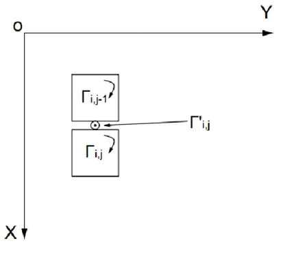
Note that the control point to which we assign the 𝛤′𝑖,𝑗 in the middle of the line is what the two control points 𝑖, 𝑗 and 𝑖, 𝑗 − 1 Figure 17. Are the normal and tangential vectors, with respect to the angle of incidence, as measured in the 𝑂𝑋𝑌𝑍 reference frame.

Pressure type Kutta condition

GPP, MPP and VLWU codes

Basic modules of the code

Type base vector: we name this object as "base_vectors" and it has three type vector objects: e1, e2, e3.

GPP and MPP code

Its main purpose is to store the orthogonal basis of the 3D space at any time. The amplitude, phase, and chordwise pitching axis position of the pitch motion. This subroutine generates the motion and the new positions of the wing at each time step.

This subroutine performs the rearrangement of the wing mesh nodes in such a way that the subroutine write_system_geometry_at_time_t can export the file needed by the VLWU code. This subroutine creates an output file in the specified format to be used as the import file for the VLWU code. This subroutine creates an output file in a special format to be imported into TECPLOT software for wing motion animation.

The VLWU code

This subroutine reads all wing positions at each time step as generated by the GPP and MPP codes. This subroutine performs the inverse of the creat_c0_t subroutine mentioned in the previous section. The difference between this subroutine and the one in Section 3.2.6 is that in addition to the wing geometry, the time-evolving track geometry is also exported to be visualized by the TECPLOT software.

This subroutine calculates the induction factors at a point A from a line vortex starting at point B and ending at point C. These subroutines calculate the velocities of the sinusoidal gust, pitch and heave motion at a point on the wing.

Presentation of results

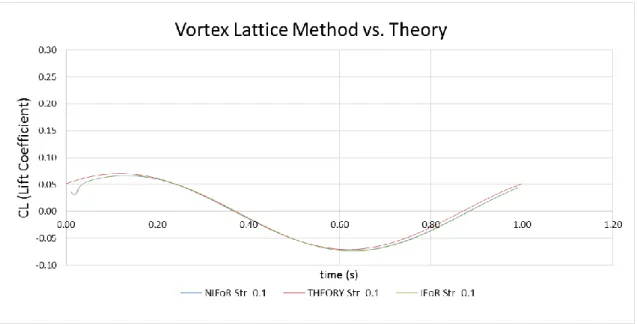
VLWU code vs Theoretical data

Finally, the lift coefficient at the center of the wing is compared with the theoretical solution. 76 c) The largest deviation between theory and VLMU can be observed near the time 𝑡 = 0 and especially at the beginning of the simulation with the VLWU method. This is due to the breakout starting at the first time steps of the simulation, as a strong initial vortex is generated near the trailing edge.

In this case, the additional fact that the pitching axis is at half the chord length of the wing has been used. In this section, we will examine what influence the mesh discretization has on the solution of the problem. The same conclusions can be drawn for the rest of the cases (ie heave and pitch motion).

As the above diagram shows, the accuracy of the solution increases as the number of panels increases, which was an expected result. In this section we will investigate the influence of the discretization of time on the solution of the problem. In this section we investigate how the wing span can influence the solution.

Wake visualization

The shape of the wake panels that do not fit on the Kutta strip remains "frozen" in space. The final model allows a certain deformation of the track according to some controlled parameters that are determined heuristically. In this section, we will use TECPLOT software to visualize the furrow shape in all movements.

This is something you would expect since we have implemented a frozen wake model where the induced surface velocities of the wake on itself are not taken into account. Finally, the time evolution of the following graphs goes from the upper left to the upper right direction and from the lower left to the lower right direction. We will observe wake roll-up at the edges of the shear layer and roll-up.

In all the above diagrams we can see the deformation of the wave and the rotation of the wake at its edges. Wake swirl are vortices that emerge from the wingtip and dissipate over time, these vortices are known as wingtip vortices and are a real phenomenon observed in nature, Figure 40. Modeling the wake as a free shear layer it is of great importance to understand the nature of awakening and the phenomenon as a whole.

Conclusions and future work

Alatzatianos, Unsteady nonlinear flow around a 2-D airfoil with free wake using the vortex grid method. Calculation of performance and cavitation characteristics of propellers, including effects of non-uniform flow and viscosity. Alatzatianos, Unsteady lifting surface method for a propeller, unsteady linear theory of two-dimensional hydrofoil (Greek).