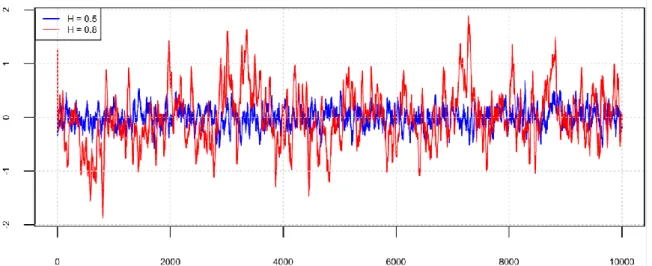
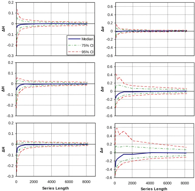
[PENDING] Use of Bayesian techniques in hydroclimatic prognosis

Mean value of ΔH and Δσ (left) and their respective standard deviations from 200 groups of 128 long synthetic time series (right) versus q, where ΔH = H^ - H, Δσ = σ^ - σ, τH. Summary results for AR(1) and HK case parameters in the Boeoticos Kephisos River Basin.

Introduction

Long horizons of prediction within a stochastic framework
Long-term persistence in predicting the climate
A Bayesian framework on the prediction of climate
Objectives and research questions .1 The broader perspective
Thesis outline

An important consequence is that to calculate π(θ|x1:n) the calculation of the integral term is not necessary. How can the uncertainty in the estimation of the parameters be integrated into the uncertainty of the prediction.

Figure 1.1. Moving average for 30 points for a simulated HKp with μ = 0, σ = 1 and (a) H = 0.5 and (b) H = 0.8

An algorithm to construct Monte Carlo confidence intervals for an arbitrary function of probability distribution parameters

Introduction

An algorithm for constructing Monte Carlo confidence intervals for an arbitrary function of probability distribution parameters. We then generalize this new algorithm to construct confidence intervals for the parameters or functions of parameters for multi-parameter probability distributions.

Terminology and notation

Construction of confidence intervals for one-parameter distributions

Now it is clear from (i) above that the confidence interval obtained from (2.17) is an exact confidence interval. b) For scale families, the quantity σ/σ (where σ is an MLE of the location parameter σ) is a key quantity (see Lawless 2003 p.562). Now it is clear from (ii) above that the confidence interval obtained from (2.17) is an exact confidence interval.

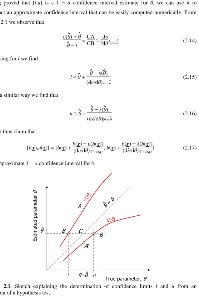
Figure 2.1. Sketch explaining the determination of confidence limits l and u from an inversion of a hypothesis test

Construction of confidence intervals for multi-parameter probability distributions We assume now that we have a multi-parameter probability distribution with density f(x|θ)

In Section 2.7 we show that the confidence interval for the parameter μ of a normal distribution N(μ,σ2) is asymptotically equivalent to a Wald-type interval. We also show that the confidence interval obtained by our method is asymptotically equivalent to a Wald-type interval for two-parameter regular distributions and thus for any multiparameter distribution.

Simulation results

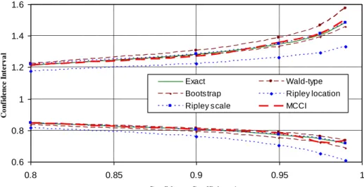
The confidence interval obtained by (2.48) is exact, and the confidence interval obtained by (2.46) is of the Wald type. These two are also compared to each other with the non-parametric BCa bootstrap bootstrap interval labeled as "bootstrap", the two confidence intervals obtained by Ripley's two methods labeled "Ripley's location" and "Ripley's scale" respectively, and the confidence interval obtained by our algorithm labeled as MCCI (Monte Carlo Confidence Interval). In this case, we use unbiased estimators μ and σ2 (instead of MLE) to calculate the confidence interval.

First, we show how we can calculate an approximate confidence interval for the scale parameter of the gamma distribution. We denote the confidence region obtained by (2.68) and (2.69) as Bayesian, the interval BCa as "bootstrap", the confidence interval obtained by two Ripley methods as "Ripley's location" and "Ripley's scale", and the confidence interval obtained by our algorithm as MCCI.

Figure 2.2. Confidence intervals for the scale of an exponential distribution with n = 50, σ ^ = 1.002

Sensitivity to the choice of the increment and the simulation sample size

MCCI was better at estimating the confidence intervals for the normal and gamma distribution parameters and had the best mean rank for all the cases studied. Monte Carlo coverage probabilities and ranking of each method by calculating 0.975 confidence intervals after 10 000 iterations (rank 1 is assigned to the best performing method).

Some theoretical results

We will also show that the confidence interval obtained by our method is asymptotically equivalent to a Wald-type interval for two-parameter regular distributions.

Figure 2.10. 0.95 confidence intervals for a normal distribution estimated for different δμ and δσ (the parameter increments denoted in text as δθ i ): (upper) confidence interval for the location parameter μ from a sample with n =

Application of the algorithm to a historical river flows dataset

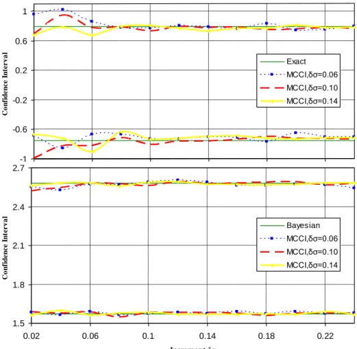
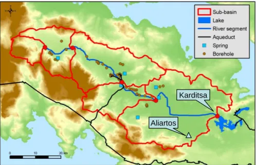
The case study is carried out on an important basin in Greece, which is currently part of the water supply system of Athens and has a history, in terms of hydraulic infrastructure and management, going back to at least 3500 years ago. The example presented in Figure 2.12 is for the January monthly flow record at the Boeoticos Kephisos river outlet at the Karditsa station measured in hm3. Here we derived confidence intervals for the scale and the shape parameters of the gamma distribution.

Comparison of the results of the different methods used shows that the MCCI and "Ripley scale" limits are close to the Bayesian. In addition, Figure 2.13 gives confidence limits of the distribution percentiles using the same data set, this time compiled with Hydrognomon (Itia research group.

Conclusions

In addition, Figure 2.13 shows the confidence limits of the distribution percentiles using the same dataset, this time constructed using Hydrognomon (Itia research group 2009-2012). We propose the use of the algorithm for an approximation of a confidence interval of any parameter for any continuous distribution, because in each case it is easily applicable and gives better approximations than other known algorithms, as shown above in specific cases. An additional advantage over Ripley's two methods is that it is not necessary to select one of the methods.

The confidence intervals obtained by the algorithm are approximate, and the algorithm is not designed with the intention of replacing the exact confidence intervals when their calculation is possible. Further research is needed to evaluate the influence of the choice of the numerical parameters (increments δθi and the simulation sample size) on the results of the algorithm.

Figure 2.12. Confidence intervals for the scale (upper) and shape (lower) parameter of a gamma distribution, used to model the Boeoticos Kephisos river January monthly flows with n = 102, α ^ = 3.842 and σ ^ = 15.218

Simultaneous estimation of the parameters of the Hurst-Kolmogorov stochastic process

Introduction
Definitions
Proof of equations (3.6) and (3.8) From equation () we obtain
Proof of boundedness of the LSV estimate of H in (0, 1]
Calculation of Fisher Information Matrix’s elements
Results
Conclusions

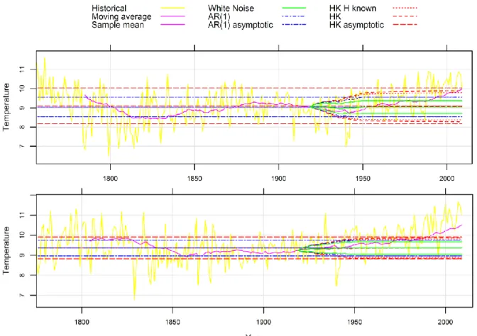
The ML method estimates the Hurst parameter based on the entire structure of the process, that is, in this section the maximum likelihood method is used for the estimation of the parameters of HKp, namely H, σ, μ. This is the basis to form a modified version of the LSSD method, the LSV method.

Average of the estimated ΔH and Δσ (left) and their corresponding standard deviations from 200 ensembles of synthetic time series 128 long (right) versus q, where ΔH = H^ − H, Δσ = σ^ − σ, τH and τσ are standard deviations and p = 6 for the LSV estimator. The choice of p must take into account the conflicting criteria of minimum bias and minimum variance of the estimator.

Figure 3.1. Monte Carlo confidence intervals for the H and σ estimates with true H = 0.60, H

The predictive distribution of hydroclimatic variables

Introduction

To this end, we solve the problem of climate predictions of natural processes using Bayesian statistics, instead of the stochastic framework developed by Koutsoyiannis et al. We derive the posterior predictive distribution (Gelman et al. 2004 p.8) of the process in closed form given the posterior distribution of the parameters. Additional results such as the posterior distributions of the parameters and the asymptotic behavior of the predictive distribution are also given.

Here we provide posterior predictive distributions of climate variables, while Koutsoyiannis et al. 2007) provide confidence limits for specific quantiles of climate variables. The posterior predictive distribution of the variables given here is exactly what we call a climate prediction, while the confidence limits of the quantiles given by Koutsoyiannis et al. could be said to be. 2007), are intermediate or indirect results.

Based on the time dependence of the processes, three alternative assumptions are given: a) independence in time; (b) Markov dependence modeled by a first-order autoregressive procedure (AR(1)); and (c) dependence on HK (for a justification of the latter, see Markonis and Koutsoyiannis 2013). Although this chapter uses the same case studies as those in Koutsoyiannis et al. 2007), the results are not directly comparable. The Bayesian methodology used here aims at (stochastic) prediction (Robert 2007, p. 7) and is straightforward, while its disadvantage compared to Koutsoyiannis et al. 2007) much higher computational burden.

The autocorrelation ρ|i−j| This is assumed to be a function of a parameter (scalar or vector) φ, so that θ := (μ, σ2, φ) is the parameter vector of the process.

Posterior predictive distributions

When looking for the asymptotic behavior of the process, (4.18) still holds after small modifications, according to Horrace (2005). We implement the algorithm using the function MCMCmetrop1R in the R package 'MCMCpack' (Martin et al. 2011). The diagnostics of Heidelberger's method provide an estimate of the number of samples that should be discarded as a burn-in sequence and a formal test for non-convergence.

When calculating the test statistic, the spectral density is estimated from the second half of the original chain. If the null hypothesis is rejected, the first 0.1n of the samples are discarded and the test is re-applied to the resulting chain.

Mathematical proofs

Case studies

In the second case, the update is done excluding the last 90 years of the datasets (C6, C7). To simulate from (4.7) for the φ1 and H posterior distribution of the AR(1) and HK cases correspondingly, we used a. Summary results for the parameters of the AR(1) and HK cases respectively are shown in Table 4.8 and Table 4.9.

A summary of the results for the parameters of the AR(1) and HK cases is shown in Table 4.8. The posterior distribution of σ is also wider on the right (see the 0.975 quantile values in Table 4.8 and Table 4.9) for HKp.

Figure 4.1. The Boeoticos Kephisos River basin.

Summary

In C5 and C7, HKp appears to be the best model as it captures better than the others the observed values of the climate variable for the last 90 years based on the observed values of previous years. We derived the posterior distributions of the model parameters, the posterior predictive distributions of the process variables, and the posterior predictive distributions of the 30-year moving average, which was the climate variable of interest. However, the posterior distributions of the means are wider when using HKp due to process inertia and even wider when all process parameters are assumed to be unknown.

Summary results for the parameters of the AR(1) and HK cases in Berlin and Vienna, respectively. Work on the generalization of the methodology for integrating deterministic forecasts with climate models is presented in Chapter 5.

Figure 4.11. Historical climate and confidence regions of climate (for 1 − a = 0.95 and climatic time scale of 30 years) for (upper) temperature at Berlin/Tempelhof after the year 1920 and (lower) temperature at Vienna after t

On the prediction of persistent processes using the output of deterministic models

Introduction
Maximum likelihood estimator for the parameters of the bivariate HKp
Posterior predictive distributions
Case study
Summary and conclusions

95% confidence region for the predicted 30-moving mean temperature (°C) for the A1B scenario of the ECHO-G model, using the NOAA annual global land and ocean temperature anomalies. 95% confidence region for the predicted 30-moving mean temperature (°C) for the B1 scenario of the ECHO-G model, using the NOAA annual global land and ocean temperature anomalies. 95% confidence region for the predicted 30-moving mean temperature (°C) for the A2 scenario of the ECHO-G model, using the NOAA annual global land and ocean temperature anomalies.

95% confidence region for the 30-run forecast mean temperature (°C) for the A1B scenario of the CGCM3.1 (T63) model, using the combined CRU land [CRUTEM4]. 95% confidence region for the 30-moving mean forecast precipitation (mm) for the A1B scenario of the ECHO-G model, using CRU precipitation over land surfaces.

Figure 5.1. Scetch explaining the time periods that are used for model calibration, i.e

Summary, conclusions and recommendations

Methodological contributions

In Chapter 3, a simulation study was conducted to assess the performance of different estimators of the HK process. The posterior distributions of the model's parameters, the posterior predictive distributions of the process variables, and the posterior predictive distributions. In the cases studied, it performed well and was able to explain the fluctuations in the process.

Posterior distributions of the parameters were derived and were shown to be wider for HKp. This meant that the output of the GCM had no effect on the stochastic predictions.

Recommendations for further research .1 Technical issues

Limitations

Engelhardt M, Bain LJ (1978) Construction of optimal unbiased inference procedures for the parameters of the gamma distribution. Maximum likelihood estimates of the parameters of the bivariate HKp for the GISS global land-ocean temperature index. Maximum likelihood estimates of the parameters of the bivariate HKp for NOAA annual global land and ocean temperature anomalies.

Maximum likelihood estimates for the parameters of the bivariate HKp for the CRU combined land [CRUTEM4] and marine temperature anomalies. Maximum likelihood estimates for the parameters of the bivariate HKp for the CRU precipitation over land areas.