The objective of this study is to determine the best value-at-risk (VaR) model for the major US stock indexes. We use historical simulation and variance-covariance approach with estimated volatility from moving average, exponentially weighted moving average, GARCH (1,1) with normal distribution, GARCH (1,1) with Student-t distribution, EGARCH (1,1) with normal distribution distribution and EGARCH (1,1) with Student-t distribution. Our results show that the most accurate results are obtained when using the Student's t-distribution together with a volatility forecasting model that takes into account the leverage effect, such as EGARCH (1,1).
Introduction
2 According to Christoffersen (2012), VaR is a simple measure of risk that answers the following question: What loss is such that it will only be exceeded 𝑝 × 100% of the time in the next K trading days. The daily revaluation of a position held by the company has also resulted in the need for a more frequent assessment of the market risk on this position. An important advantage of the RiskMetrics method is the presentation of the measurement of the market risk as a single number, which has been very useful and easy to understand for investors.
There are two main reasons for this: first, the historical data of the security in question must be used to calculate VaR, and historical data does not always correspond to current data. After the collapse of many financial institutions, such as Lehman Brothers, one of the largest investment banks in the United States, the measurement of market risk was once again put to the test. The rest of the thesis is structured as follows: Section 1 provides the background of VaR as a measure of risk.
Literature Review
This result is exclusive to the stock market data, as GARCH (1, 1) did not have the best predictions for the other types of markets (3-month Treasury bill yield, 10-year Treasury bond yield and Deutschemark exchange rate) . Statistical and operational evaluation of these models showed that the moving average and the GARCH gave the best results for all the stock indices except for the US index. The results show that for the 97.5% confidence level most of the models indicate good outcomes, with GARCH (1, 1), EGARCH (1, 1) and TARCH (1, 1) performing better for the long positions.
For the 99% confidence level, the filtered historical simulation method showed the best results and acceptable extreme value theory results. The stock portfolio analysis results for the HS and MC simulations show that for the 99% confidence level, all methods are acceptable and can be included in the BIS 'green' zone. The authors believe that the widespread use of these very popular models was the reason for the underestimation of risk in financial institutions in the recent crisis.
Theoretical Framework
- Advantages and disadvantages of VaR
- Stylized facts
- Normal Distribution
- Student-t Distribution
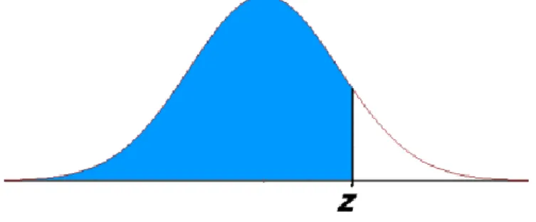
VaR has many advantages, making it one of the most popular risk measures used worldwide. This should be even clearer because of the short horizon that we will use (on a daily basis). The shape of the normal distribution is a bell curve and is one of the most important distributions in statistics.
The standard deviation determines the shape of the distribution, if it is spread out, or if the majority of the surface will be concentrated near the top. 12 It also provides the area under the density function of the standard normal random variable, which is to the left of the specified value 𝑧. As they decrease, they diverge from the shape of the Normal Distribution by demonstrating lower peaks and fatter tails.
Methodology for calculating VaR
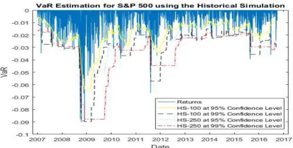
Historical Simulation
Then the returns within this window are sorted in ascending order and the value that leaves 𝑝% of the observations on its left and (1 − 𝑝)% on its right is the VaR. To calculate the VaR the next day, the entire window is moved forward by one day and the entire procedure is repeated. The historical simulation is easy to implement, but has been criticized mainly for using past data when predicting the future.
Parametric method – Variance / Covariance Matrix
- Markov Process
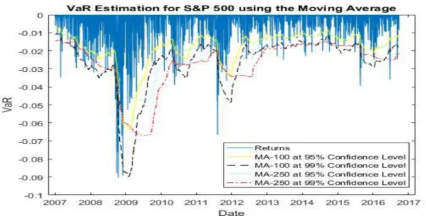
- Ways for estimating volatility
A variance level of 1 means that the variance of the change in 𝑧 in a time interval of length 𝑇 is equal to 𝑇. This tells us that the distribution of an asset's returns will depend entirely on the asset's volatility. This means that the conditional volatility of the financial series evolves according to an autoregressive type process.
Specifically, ARCH models assume that the volatility of the current error term is a function of the previous one. This equation states that the conditional volatility of a zero mean normally distributed random variable 𝑦𝑡+1 is equal to the conditional expected value squared 𝑦𝑡+1. In this case, ℎ𝑡+1 is calculated from the first recent estimate of the volatility rate and the first recent observation on 𝜀2.
Backtesting
Unconditional coverage testing
We first want to test whether the violations obtained from a particular risk model are significantly different from the coverage ratio 𝑝. This test is about whether the expected VaR is violated more (or less) than 𝑝 ∗ 100% of the time. As the number of observations 𝑇 goes to infinity, the test is distributed as a 𝜒2 with one degree of freedom.
This likelihood ratio, or equivalently its logarithm, can then be used to calculate the 𝑝-value, or compared to a critical value using a significance level to decide whether to accept or reject the null hypothesis. 26 refers to the possibility of rejecting the correct model, and type 2 error refers to the possibility of not rejecting (accepting) the incorrect model. This can be interpreted in one of two ways: if 𝜋 > 𝑝, losses exceeding the predicted VaR occur more often than 𝑝 ∗ 100% of the time.
This would suggest that the forecasted VaR measure understates the portfolio’s actual level of risk. The opposite, 𝜋 < 𝑝, would mean that the VaR measure is conservative and overestimates the risk.
Independence testing
28 If the probabilities are independent over time, then the probability of a violation tomorrow does not depend on whether or not there is a violation today, so 𝜋01 = 𝜋11 = 𝜋. We use the 𝑝 value or the critical value to determine whether to accept or reject the hypothesis.
Conditional Coverage Testing
Data
Out of sample period, which we will use in backtesting to compare forecasts with realized returns and to determine the accuracy of the methods used. Having chosen 2007 as the starting point in our study, it coincides with the onset of the most recent financial crisis which also began in the summer of 2007. All indices except the DAX and CAC are negatively skewed, meaning that the tail of the left side of the distribution is longer than the right side.
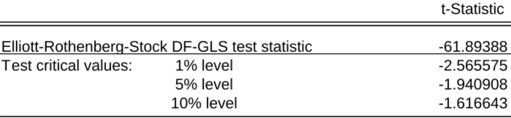
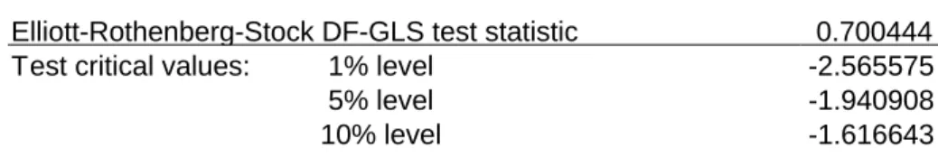
The kurtosis is more than 3 for all the indices, indicating a leptokurtic distribution, which is characterized by fatter tails. The probability measure is 0.00 for all the indices, causing the rejection of the hypothesis for normality. We performed the ADF-GLS unit root test to determine the stationarity of the time series.
As we can see from the tables 11-24 in Appendix A most of the time series show the presence of unit root in the level. On the other hand, when using the 1st difference of the time series in the test, the unit root does not exist, and instead the time. This fact validates the use of the logarithmic differences instead of the price levels in all of the models.
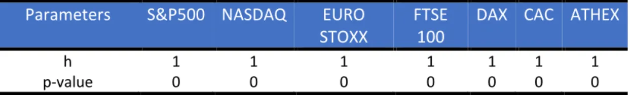
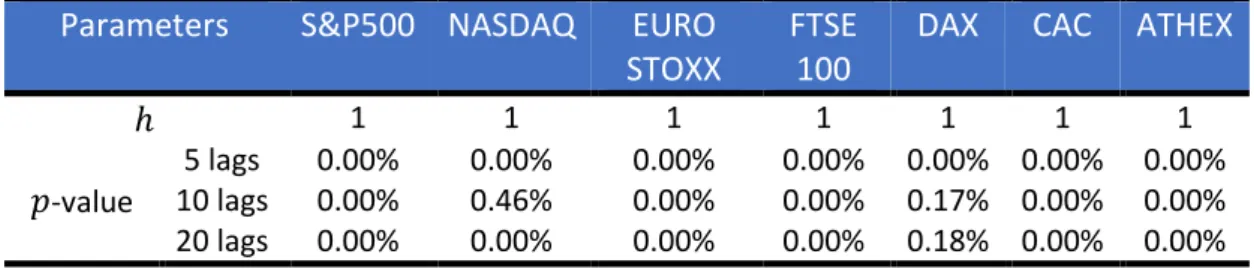
A logical value (ℎ) of 1 indicates the rejection of the null hypothesis for no autocorrelation, ℎ = 0 indicates the non-rejection of the null hypothesis. For all the indices, the test indicates the rejection of the null hypothesis H0: no autocorrelation. All the logic values indicate the rejection decision and all the 𝑝 values are less than 10% for all the delays reported.
Appendix Section B2 presents sample ACFs and PACFs of squared returns (Figures 10-16).
Empirical Findings
- S&P500
- NASDAQ
- EUROSTOXX
- FTSE100
- DAX
- CAC
- ATHEX
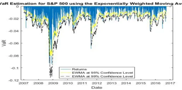
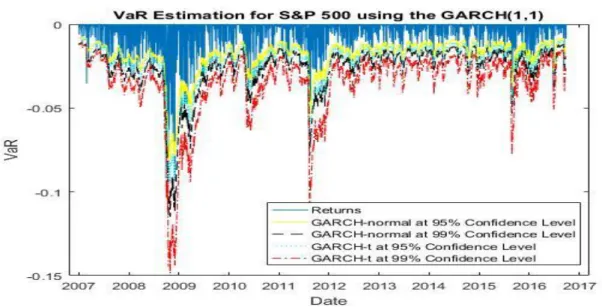
At the 95% confidence level, the highest number of violations is made using EGARCH (1,1) with a normal distribution (170) and the lowest number with GARCH (1,1) with Student's t-distribution (103). At the 99% confidence level, the highest number of violations is made using a moving average with 250 observations (76), and the lowest is made using GARCH (1.1) with Student's t-distribution (17). Closest to the expected number of violations is the EGARCH (1,1) with Student's t-distribution (30 with an expectation of 25).
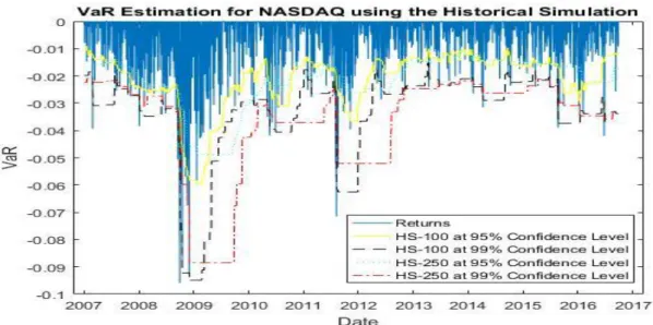
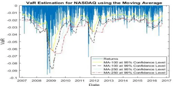
At 95% confidence level, the highest number of violations is made using EGARCH (1,1) with normal distribution (159) and the lowest number was with GARCH (1,1) with Student's t-distribution (112). At 95% confidence level, the highest number of violations is made using EWMA (157) and the lowest number using GARCH (1,1) with Student's t-distribution (107). Again, closest to the expected number of violations is EGARCH (1,1) with Student's t-distribution (128 when 123 is expected).
At 95% confidence level, the highest number of violations is made using EWMA (166) and the lowest number with GARCH (1,1) with Student's t-distribution (114). Again, the closest to the expected number of violations is EGARCH (1,1) with Student's t-distribution (131 when expecting 123). Again, very close to the expected number of violations is EGARCH (1,1) with Student's t-distribution (26 when expecting 25).
At 95% confidence level the highest number of violations is made using Exponentially Weighted Moving Average (160) and the lowest using GARCH (1,1) with Student’s t- distribution (112). The closest to the expected number of violations is the EGARCH (1,1) with Student’s t-distribution (134 when expecting 125). At 99% confidence level the highest number of violations is with the Moving Average with 250 observations (60) and the lowest number with GARCH (1,1) with Student’s t-distribution (16).
At 99% confidence level the highest number of violations is made using the Moving Average with 250 observations (57) and the lowest using GARCH (1,1) with Student’s t-distribution (20).
Conclusion
If we were less conservative and chose a 5% level for the 𝑝 value, it would pass all the tests in all the indices. In almost all cases, it predicted the exact number of violations as expected. On the relationship between the expected value and the volatility of the nominal premium on shares.
We compare the absolute value of the t-statistic with the critical test values at 1%, 5% and 10% levels.
S&P 500
NASDAQ
EUROSTOXX
FTSE
DAX
CAC
ATHEX