A Generalized Wave Field Synthesis Framework

The current dissertation reviews the theoretical foundations of Value Field Synthesis in order to overcome the limitations of previous approaches. I am especially grateful to Frank Schultz for friendly and fruitful discussions, all cooperation and for careful proofreading of this dissertation.

Overview of spatial audio techniques

The latter is discussed within the context of the proposed theoretical framework in the present thesis. Since WFS provides driving signals of the local behavior of the virtual sound field at the position of the loudspeakers, it is often labeled as a local solution to the SFS problem.

Figure 1.1. Typical two-channel stereophonic loudspeaker geometry (a) and exemplary interchannel amplitude and time differences (b) for the panning of the phantom source to be localized from the angular direction φ p

Wave Field Synthesis history and motivation of the presented research: 6

The homogeneous wave equation

The relative change of volume dV /V0 can be expressed by the divergence of the particle displacement ∇x u(x, t). By taking the time derivative of equation (2.4) and the divergence of equation (2.1), the particle velocity can be eliminated.

The inhomogeneous wave equation

In addition to the pressure and velocity, acoustic fields are often described by the scalar velocity potential ϕ(x, t), for which the acoustic wave equation also applies, and which is related to the other field variables such as To involve more physical source excitation models, additional power source terms can be added to the equation of motion (2.1) or injected mass/volume terms can be included in the continuity equation (2.4).

Boundary conditions

The Sommerfeld radiation condition can be derived in a mixed internal and external radiation problem by prescribing appropriate boundary conditions on the surface∂Ω∞in addition to increasing its radius to infinity, ensuring that no reflection can occur from this external boundary surface. These types of boundaries are called rigid, orrigid soundings, with the boundary condition ensuring that no incident wave can mobilize the boundary surface.

Solution of the homogeneous wave equation

Plane wave theory

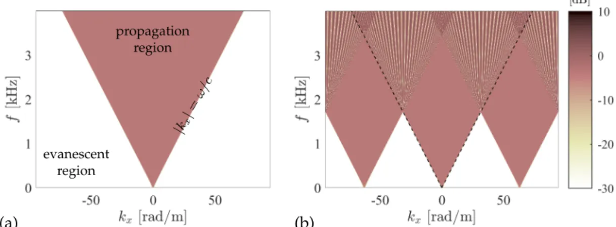
For the evanescent wave case, kx > ωc, causing an exponential decay along their direction. In the source-free region, propagating and escaping waves form a complete, orthonormal basis for solving the Helmholtz equation.

Figure 2.2. Illustration of a traveling plane wave (a) and an evanescent wave (b) with λ = 2π k being the acoustic wavelength of the plane wave

The angular spectrum representation

The evanescent contribution is often neglected in the field of sound field synthesis when the listener is relatively far from the array of secondary speakers and the speaker spacing is significantly greater than the evanescent wavelengths. Formulating the equations in the spatial domain results in 2D spatial convolutions called Rayleigh I and II integrals, as discussed further in the following sections.

Solution in other geometries

These statements lead to two important formulations: Equation (2.31), written in the spatial domain by means of a double inverse Fourier transform, gives. 2.33) By expressing P˜(kx, y0, kz, ω) in terms of the normal velocity V˜n(kx, y0, kz, ω) using the Euler equation (2.8), with the calculated normal (y-) derivative aty=y0 using the differentiation theorem we get Wave propagation is calculated by multiplying the measured spectra with an exponential term called the pressure propagator G˜p v (2.33) and the velocity propagator G˜v v Wave propagation in source-free volumes can thus be modeled by 2D linear spatio-temporal filtering of the sound field measured along a plane , where the transfer characteristics of the filter are given by the corresponding propagator.

Solution of the inhomogeneous wave equation

The Green’s function

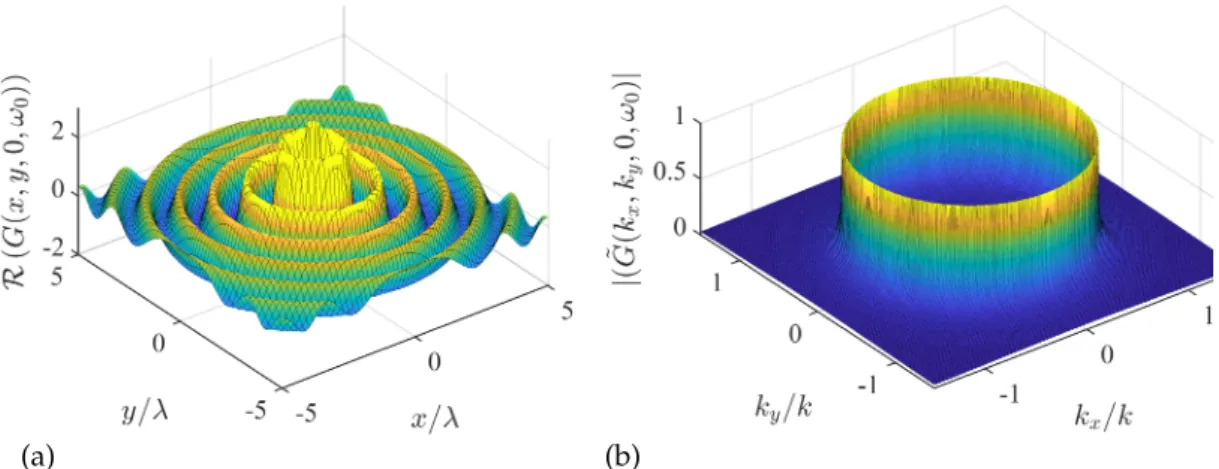
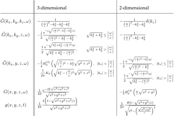
Applying the Fourier convolution theorem to (2.41), the solution of the inhomogeneous wave equation (2.10) in the wavenumber domain reads as. Different representations of the 3D free field Green's function in the angular frequency domainG(x, y, z, ω), withλ= 2πcω =2πk (a) and in the semi-wavenumber domain (i.e. the angular spectrum)G(k˜ x) , ky , z, ω)metk= ωc (b), measured atz= 0.

Table 2.1. Free field acoustic Green’s function representations ( x 0 = 0 ) [DeS92; Duf01; Gib08;

Solution of the general inhomogeneous wave equation

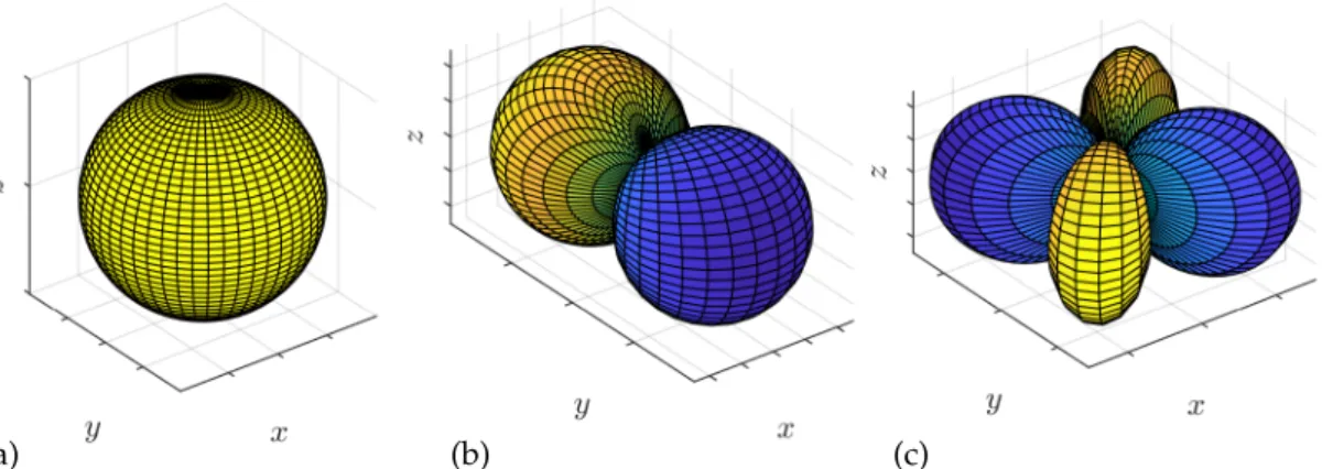
Qualitative illustration of the directional characteristics of a monopole (a), a dipole with the axis of the dipole being their axis (b), and a horizontal quadrupole constructed from two opposite dipoles in the horizontal plane (c). In the figures, the distance from the origin indicates the absolute value of the direction in the given direction, with the sign indicated by the color of the surface.

Figure 2.4. Qualitative illustration of the directivity characteristics of a monopole (a), a dipole with the dipole axis being the y axis (b) and a horizontal quadrupole constructed from two opposing dipoles in the horizontal plane (c)

Boundary integral representation of sound fields

The Kirchhoff-Helmholtz integral equation
The simple source formulation
The Rayleigh integrals
The local wavenumber vector
The local wavefront curvature
High frequency gradient approximation

It is now investigated how the wave dynamics can be described in terms of the local wavenumber vector. In the next section, the physical interpretation of this equation is explored in terms of the local wavenumber vector and the local curvature of the wavefront.

Figure 2.6. Illustration of the simple source formulation in a 2D interior problem ( Ω ⊂ R 2 ).

The Kirchhoff approximation

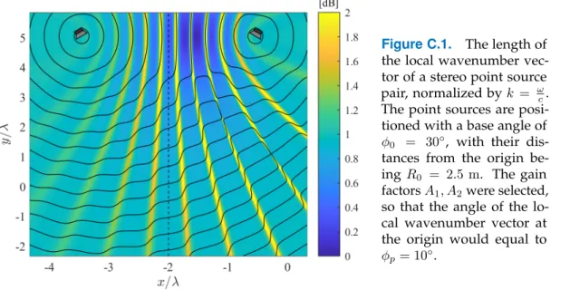
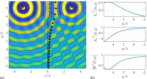
The amplification factors A1, A2 were chosen so that the angle of the local vector of the wave number at the origin was equal to φp= 10◦. Figure (b) describes the total field of a point source in the presence of a sound-scattering object.

The stationary phase approximation

The integral approximation

Moreover, in the vicinity of the stationary point A(x) can be considered constant, with the value A(x∗). In the following, the physical interpretation of SPA when applied to boundary and spectral integrals of sound fields is discussed and simple examples are given for its application.

Asymptotic approximation of boundary integrals

According to definition (3.2), the derivatives describe the corresponding components of the local vector of wavenumbers. Therefore SPA 'compares' the direction of propagation/wavefront of the described field and the Green's function along the integral path.

Figure 3.7. 2D Geometry for the physical interpretation of the station-ary position for the Rayleigh integral.

Asymptotic approximation of spectral integrals

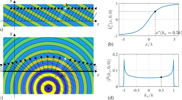
Interpretation of the spectrum of the Green's function as the field of a line source, with harmonic spatial distribution, described by wavenumberkx, evaluated atx= 0. The high-frequency approximation of the 2D Green's function - which therefore arises from the asymptotic approximation of (2.46) [ Wil99, p. The drive function (4.4) is a general generalization of the 3D WFS control function given by [ZS13, (20)] specific to a virtual point source.

The drive function ensures amplitude-correct synthesis within the validity of the Kirchhoff approximation: amplitude errors occur.

Figure 3.9. Illustration of the stationary position for the SPA of the Fourier transform in case of a 3D point source, with its one-dimensional Fourier transform evaluated along the x -axis.

The 2.5D Kirchhoff approximation

Within the validity of SPA, the driving function (4.14) ensures amplitude-correct synthesis in the reference position. Due to the phase characteristics of the Green's function, the reference position xref(x0) for any SSD element can be found at the intersection of the reference curve and the line originating from x0 pointing to the local wavenumber vector of the virtual field kP(x0). The reference position location for a given SSD element is shown in Figure 4.4 for the virtual point source example.

Taking the time-inverse Fourier transform of the driving function weighted by S(ω), we obtain the time driving function for a virtual point source with source time history s(t).

Figure 4.3. Geometry for the derivation of 2.5D Kirchhoff in-tegral. The enclosing surface

Explicit solution: Spectral Division Method

Explicit solution in the spatial domain

With these considerations and by expressing the second derivatives in terms of the principal rays according to (B.6), the explicit row function takes its final form. The formulation implies the fact that, as with the implicit solution, the explicit control function also requires the derivative of the target field measured at the reference position. The drive function includes a virtual source compensation factor, which compensates for the relative amplitude change of the virtual sound field between the SSD and the reference curve in terms of the principal horizontal ray.

In the following, a simple example is presented to demonstrate the validity of the spatial SDM driving function for the synthesis of a virtual 3D point source.

Figure 4.10. Illustration of the stationary position x ref (x 0 ) for the evaluation of the spatial ex-plicit driving function

Relation of implicit and explicit solutions

Although the above driving function is derived from the pressure measured along the reference curve, (4.60) is already simply written in terms of the target field measured at the secondary sources, equivalent to the WFS solution. In the following, this relation is generalized by expressing the explicit driving function for an arbitrary target sound field, written in terms of the pressure measured along the SSD, revealing the general relation of the implicit and explicit solutions. However, an important difference is that the WFS driving function is obtained in an intuitive way from the 2.5D Neumann Rayleigh integral, by introducing the reference curve concept with interchanging the role of the receiver position and its stationary SSD position .

On the other hand, the clear direction function (4.53) essentially contains the horizontal SPA and the concept of the reference curve.

Synthesis applying discrete secondary source distribution

Description of spatial aliasing
Avoiding spectral overlapping
Avoiding the reproduction of mirror spectra
Time domain description
Time-frequency domain description

The wavenumber content of the synthesized field by applying a discrete SSD can be written as. 4.68). Asymmetric anti-aliasing filtering can be performed by angular low-pass filtering of the direction function according to. 4.73). In the present case the derivative of the argument (i.e. Jacobian) is expressed by applying the chain rule, resulting in

For subsonic speeds, only this positive root of the quadratic equation (τ(x, t)>0) is taken into account [Hoo05].

Figure 4.13. Illustration of the discretization process of the linear WFS driving function.

Wave Field Synthesis of moving sources

The time domain 2.5D Kirchhoff approximation

The dimensionality reduction is again performed by the stationary phase approximation of the Kirchhoff integral, resulting in the time domain 2.5D Kirchhoff approximation. The concept is illustrated in Figure 5.6 with the example of the stationary point for the field of a moving point source. Geometrically, this point lies at the intersection of the boundary and the vector pointing from the moving point source at the time of emission to the receiver position.

Calculation of the drive function requires knowledge of the emission time for each SSD element at each instant.

Figure 5.6. Illustration of the sta- sta-tionary position for the boundary in-tegral representation of the field of a moving source

Explicit solution for the synthesis of moving sources

Spectral representation of moving sources

The representation of the kx−ω domain of the field of a harmonic stationary and moving source is shown in Figure 5.10 (a) and (b), respectively. The spatial drive function is obtained from the double inverse Fourier transform of the wavenumber domain drive function. In the present case, the required wavenumber content of the virtual field is given by (5.60).

The spatial representation of the driving function is obtained by a spatial inverse Fourier transform of the above expression.

Figure 5.9. The time history and spectrum of a harmonic source moving on a trajectory x s (t) = [v · t, −2, 0] T with v = c 2 , oscillating at f 0

Practical aspects of the synthesis of moving sources

Calculation of source trajectory

Calculation of propagation time delay

Effects of the SSD discretization

The effects of the SSD discretization are illustrated in Figure 5.13 in the case of a moving source with a harmonic (a) or a broadband (b) excitation signal. Figure (a) shows the spectrum of the discretized moving source drive function with overlapping spectral repetition. Wavenumber-frequency representation of the synthesized field of a harmonically moving source, using a linear SSD (a) and the corresponding spectrogram (b).

The simulation results verify the almost full-band synthesis in the middle of the secondary array.

Figure 5.13. 2.5D synthesis of a moving 3D point source located at x s = [v · t + 1.5, −2, 0] T with v = c 2 , radiating at f 0 = 1 kHz (a), or emitting an impulse, bandlimited to 15 kHz (b)

Choosing the referencing scheme

The presented approach can be realized by simple low-pass filtering of the drive signals. The synthesis of such a converging sound field requires the correct manipulation of the stationary phase approximation. I presented how the shape of the reference curve can be controlled by applying a frequency-independent amplitude correction term to the driving function.

The derivation is based on the above equivalence of the WFS and SDM driving function.

Definition of the principal curvatures and principal directions . 133

In the aspect of this treatise, the signature and determinant of the Hessian in the stationary position is of interest. Note that the local wavenumber vector contains the amplitude of the field in its denominator. At these positions, the phase changes rapidly, resulting in an increase in the local wavenumber vector length.

The terms in parentheses cancel out due to the definition of the stationary points for the forward transformation (D.4).