10 2.1 Values of βandτfor which the limit of the duality gap decreases in LP. Interior Point Algorithms (IPAs) have been extensively studied by several authors in the last four decades and their various variants have been implemented in most commercial solvers.
Interior point algorithms
The main results regarding IPAs for LP are summarized in the books of Roos et al. In this thesis, our aim is to propose new primal dual path-following IPAs for LP problems and LCPs.
The linear programming problem
The central path problem for LP
The linear complementarity problem
The central path problem for LCPs
Main ideas of designing primal-dual path-following IPAs
The new iterates must be in a proper neighborhood of the central path so that the iteration can be repeated. We need to choose the update parameter so that the polynomial complexity of the IPA can be proven.
The algebraically equivalent transformation technique
Applying the AET technique for LP problems
Most IPAs from the literature can be considered as a special case of the AET technique with the identity function. Table 1.1 shows the values of the vector pφ and the function p(t) for the most frequently used functions from the literature.
Applying the AET technique for LCPs
Throughout the dissertation, especially in Chapter 4, we will use some important properties of p(t) to prove the correctness of the proposed algorithms. Using the same notations as in the previous section, the scaled system can be formulated as .
Literature related to the AET technique
In the case of θ = π/4 the cone reduces to the second order cone represented in the case of the SOCO problem. In the case of the LCP over the Cartesian product of circular cones (CCLCP) the goal is to determine which and which satisfy.
The method of Ai and Zhang
The decomposition of Ai and Zhang for LP problems
It is important to note that ∆x+ is not the positive part of ∆x (in this case the + sign is a subscript instead of a superscript), but it is the solution of the system with p+φ on its right-hand side. The components coming from the first system are cardinal for progress towards optimality, while the solutions in the second system have a significant role in controlling the centrality of the new iterations.
The decomposition of Ai and Zhang for LCPs
Wide neighborhood definition
Motivation, scope of the thesis 21 definition, Wf can be defined not only in the case of the identity function, but for any pas-.
Motivation, scope of the thesis
In the case of the latter function, the convergence and best-known complexity of the long-step IPA can be proven; these results are summarized in Chapter 2. We proposed a general Ai-Zhang type long-step algorithmic framework and proved that if the function applied in the AET technique belongs to a certain class of functions, then the desired properties of the general IPA can be proved.
New results
In Chapter 4, we propose a general Ai-Zhang-type long-step algorithmic framework for LP problems, where the transformation function is applied to the AET technique (more precisely, the function p(t) taken from the right-hand side of the system scale ) is part of the input. During the analysis, we consider the case of α2 = 1, i.e., we make a full Newton step in the direction (∆x+,∆s+) and determine the value of α1 in order to achieve the desired complexity of the algorithm.
Analysis of the algorithm
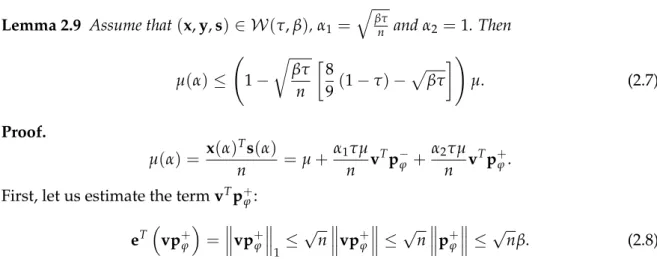
In order to prove the feasibility of the new iterations and ensure that they stay in the neighborhood W(τ,β), we need a technical lemma. The following two statements suggest limits for the duality gap at the new point, that is, µ(α) =x(α)Ts(α)/n.
Complexity of the algorithm
However, to the best of our knowledge, no algorithm in the literature combines the two approaches, i.e., Ai-Zhang type IPA using the AET technique. We apply a wide neighborhood of Ai-Zhang type, but our definition differs from (2.1) examined in the LP case.
Analysis of the algorithm
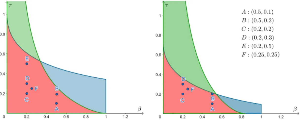
Analysis of Algorithm 41 To ensure that the iterations stay in the neighborhood WLCP(τ,β,κ), we need a lower bound on the duality gap after a Newton step. Therefore, the parameter values for which both conditions are surely satisfied (i.e., the duality gap is reduced and new iterations remain in WLCP(τ,β,κ)) are at the intersection of the two regions and are denoted by red in Figure 3.2.
Complexity of the algorithm
Convergence analysis
Here, the multiplier of µ is positive by Proposition 4.2 and it is less than one due to (C2), therefore µ(α)≤µ decreases, i.e. the duality gap. Using Lemma2.7 (the analogue of Proposition 3.2 of Ai and Zhang [4] for LP problems), we can show that the new iteratesx(α)ands(α) are strictly positive, i.e. feasible.
Complexity of the general algorithm
It follows from Theorem 4.1 that the complexity of Algorithm 4.1 is the same as in the case of fixed step lengths used in the analysis.
Constants and properties for special functions
Since this functionφ is still invertible, we can apply the AET technique by taking the right-hand derivative in formula (1.13) in the point √1. In the eleventh and twelfth rows, we have defined functions p(t) that are not strictly decreasing over [1,t∗].
Properties of the function φ
A modified AET technique with piecewise continuously differentiable
However, we could use one of the one-tailed derivatives in the definition instead, and the subsequent results would remain the same. Therefore, the AET technique using the one-tailed derivatives can be applied even in the case where the transform function is not continuously differentiable, but piecewise continuously differentiable.
Construction rules
For each i ∈ Λ, the restriction F|Ui of the mapping to each Ui is a continuously differentiable mapping. Foru=1, the statement is true since both sides of the inequality are 0 under our assumptions.
Preliminaries
Linear optimization
To be able to give strictly feasible starting points in the neighborhood W(τ,β), we first transformed the problems into symmetric form and then applied the self-double embedding technique [179]. However, in the previous chapters we assumed that the LP problem is given in standard form.
Linear complementarity problems
However, in Chapter 3 we assumed that the matrix of LCP coefficients is sufficient, or equivalently the P*(κ)-matrix. As can be seen from the pseudocode, in this case we ignore the handicap value and take the largest step so that new iterations remain in the neighborhood for κ = 0, namely inWLCP(τ,β, 0).
The role of the neighborhood and update parameters
TABLE5.6: Numerical results for the sufficient matrices generated using PSD matrices, with different parameter settings. Interestingly, the mentioned phenomenon in the case of LP problems (that the best results are obtained with the second setting) cannot be observed for LCPs in general.
Observations on LCPs with Csizmadia-matrices
Consequently, the structure of the modified LCP remains similar to the Csizmadia-LCP withq=−Me+e. FIGURE 5.3: The projection of the central path to the level of x1enx50 in the case of the 50×50 Csizmadia-LCPs withq=−Me+ηe.
Numerical results regarding the new function class
TABLE 5.12: Numerical results obtained with functions p1(t)-p10(t) using general greedy IPA for the first 26 instances of Netlib. TABLE 5.13: Numerical results obtained with functions p1(t)-p10(t) using general greedy IPA, for another 26 instances of Netlib.
Results with the theoretical step length
On the theoretical IPA for LP problems
In the case of the theoretical variant, all coordinates of v were greater than 1, that is, p+=0 held in all iterations, and the iterates never left the neighborhood N∞−(1−τ). In the case of the greedy variant, the largest coordinates were also far from the upper bound.
On the theoretical IPA for LCPs
Here, the intervals become narrower by about 2 as the algorithm progresses, and the coordinates are concentrated around this value in the end. Although this upper bound would not improve the complexity of the algorithm, it would allow proving the desired properties of the general multi-function IPA.
Testing the sufficiency of matrices
The matrix M is column sufficient if and only if the optimal objective function value of the following problem is 0. The matrix M is column sufficient if and only if the optimal objective function value of the following problem is 0 for all positiveλ.
Summary of the numerical results
Linear programming problems
Performance also depended on the structure of the problem instances; for different LP problems, different functions gave the best results. For the greedy variant, the upper bound obtained in practice is also far from the one used in the analysis and appears to be independent of the problem size.
Linear complementarity problems
Analyzing the results obtained with the theoretical step length, we found that the coordinates of the vector remain in a really narrow range if the starting point is close to the central path. To this end, we introduced a general Ai-Zhang-type long-step algorithmic framework for which the transformation function (more precisely, function p(t) describing the right-hand side of the scaled Newton system) is part of the input.
Future research
An Indeterminate Interior Point Algorithm for Path Tracking for Semidefinite Programming”. Iranian Journal of Operations Research pp.
Applications of the AET technique to different problem classes
Constants and properties for special functions
Size of the chosen LP problems and the time spent on preprocessing and post-
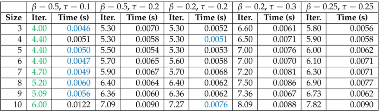
Numerical results for LP problems with different parameter settings, for the
Numerical results for the ENM sufficient LCPs with different parameter settings 73
Numerical results for the sufficient matrices generated using PSD matrices,
Numerical results for non-sufficient LCPs with different parameter settings . 74
The applied functions and parameter settings in the numerical tests for LP
Numerical results with β = 0.2 and τ = 0.1 for the chosen Netlib instances
Bounds on the coordinates of v with the theoretical IPA for LP
Average running times of BARON for sufficient matrices
Running times of BARON for Csizmadia’s matrices
Average running times of BARON for non-sufficient matrices
Outline of a general IPA for LP
We use the same notations as in the case of the SDO problem, moreover let Q∈ S⊕n be given. In the case of the SO problem, we consider a Euclidean Jordan algebra6(V,◦) where V is a vector space over Rand◦is a bilinear map.
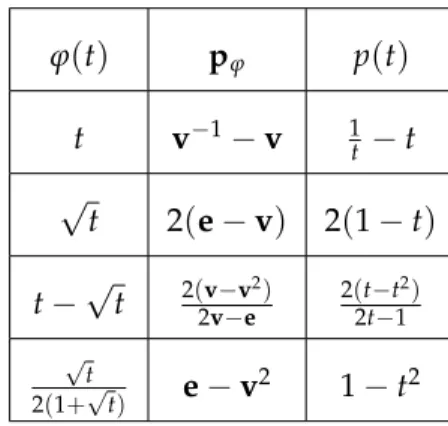
FIGURE 2.1: Values of β and τ for which the duality gap limit decreases in the LP case with φ(t) =t−√. Together with Lemma 2.10, this means that new iterations after the Newton step remain in the neighborhood of W(τ,β).
The second inequality can be verified by the property vi ≤1 when i∈ I+, and for the last estimate we used the definition of the neighborhood WLCP(τ,β,κ). The transformation function used in the AET technique (specifically, the function p(t) obtained from the right-hand side of the scaled system) is part of the input.
Outline of the general algorithm for LP problems
The following proposition will be used to prove that the reduction of the duality gap is positive. The time (in seconds) required to clean and embed the problem (preprocessing) and obtain a solution to the original optimization problem (post-solving) is also shown in Table 5.1 in columns.
Pseudocode of the greedy variant of the general algorithm for LPs
If ζ > 0, then x/ζandy/ζ are optimal solutions of the primordial and dual problems in (5.1), respectively. As already mentioned, we implemented both a greedy and a theoretical version of the general algorithm from Chapter 4.
Pseudocode of the greedy variant for LCPs
Predictor-corrector interior-point algorithm based on a new search direction working in a wide neighborhood of the central path". A new complexity analysis for full-Newton-step infeasible interior-point algorithm for horizontal linear complementarity problems".