There are infinitely many tensor product surfaces that approximate a given set of data points—the goal is to produce surfaces that are suitable for CAGD applications. At the same time, the poorly defined surfaces (see below) and the overall surface extent remain relatively small.
Previous work
- Initial data parameterization for fitting
- Constrained mesh parameterization
- Handling weak control points
- Extrapolating surface meshes
For texture mapping, position constraints must be satisfied while ensuring low geometric distortion, see [Hormann et al., 2007], Ch. The problem of weak control points (or overfitting) in the context of truncated tensor product surfaces has been studied in depth by [Weiss et al., 2002].
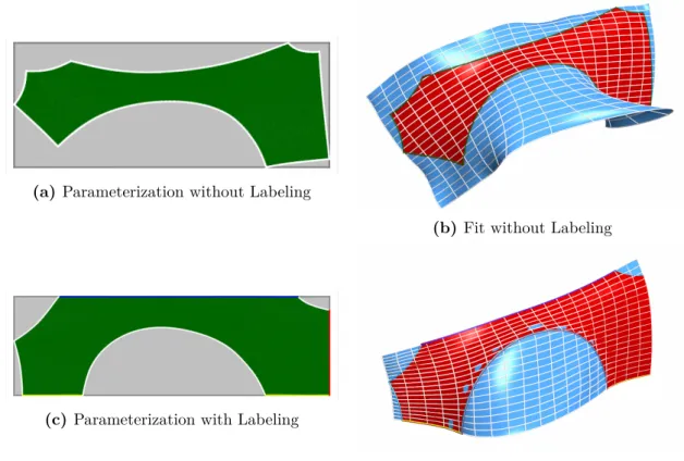
The key concept: labeling
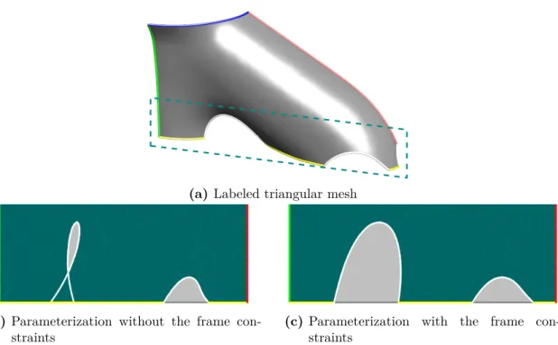
In this and the following section, labeling information will be utilized when it exists, but its meaning and origin will be disregarded. Note that while tagging is a useful technique, there are cases where it is not necessary.
Workflow
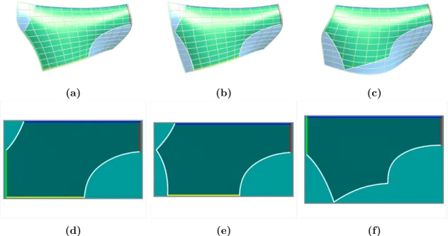
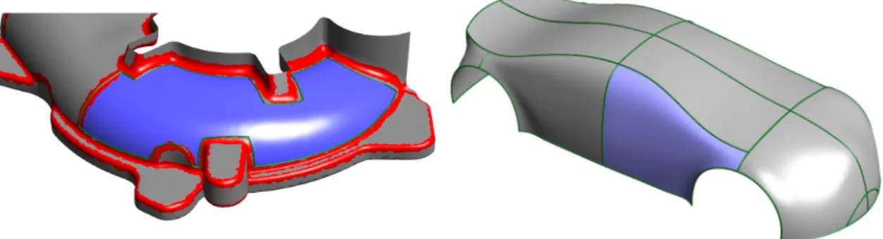
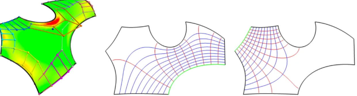
Examples include relatively flat trimmed areas or areas without umbilicals (such as swept surfaces or surfaces of revolution) where the grid of lines of curvature is not broken and an appropriate parameterization can be calculated by fitting the isolines to the grid of curvature. A counterexample is the object shown in Figure 3.8; because of its threefold symmetry and the umbilical point at the center, it would be ambiguous to fit a regular coordinate grid to the lines of curvature.
Mapping from 3D to 2D
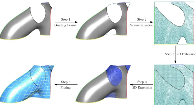
Guiding frame
A 3D guided frame is calculated, which is considered a rough approximation of the four boundaries of the surface. The guide frame is used to set the location and the relative relationship of the labeled segments.
Constrained parameterization
Mapping from 2D to 3D
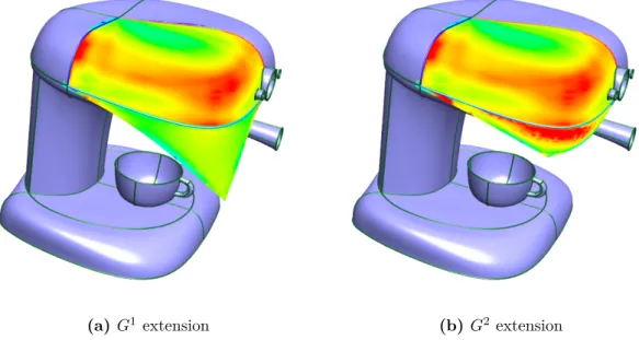
Extension in 2D
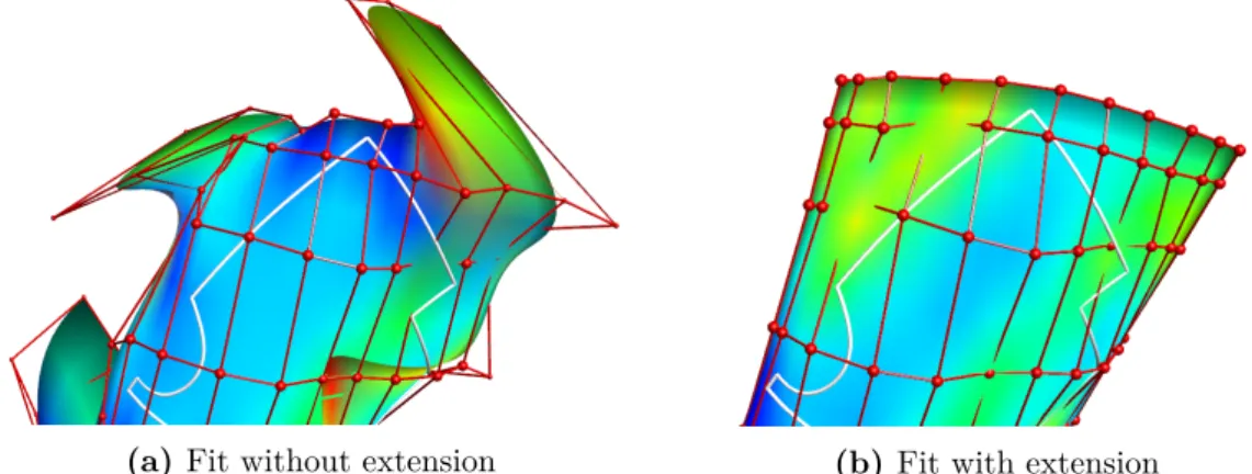
The already parameterized input data points are supplemented with new, "artificial" data points so that they fill the entire domain.
Extension in 3D
Fitting
- Summary
Labeled parameterization and extension
- Labeled parameterization
- Guiding frames
- Labeled parameterization
- Mesh extension
- Extension in 2D and triangulation
- Extension in 3D
- Discussion and results
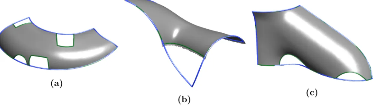
- Test cases .1 Test case 1.1Test case 1
- Parameter setting
- Details of the implementation
- Summary
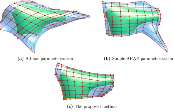
Note that the smoothness of the ARAP energy is optimized, but not its actual value. The better quality of the labeled surface is also shown by the indicators, see Table 3.2.
Automatic labeling
- Introduction
- Overview of the automatic labeling algorithm
- Detecting label candidates
- Concave angles
- Moving frame rotation
- Classifying virtual corner candidates
- Concatenating label candidates
- Removing label candidates
- Test examples
- Example 1
- Example 2
- Example 3
- Example 4
- Example 5
- Parameter setting
- Summary
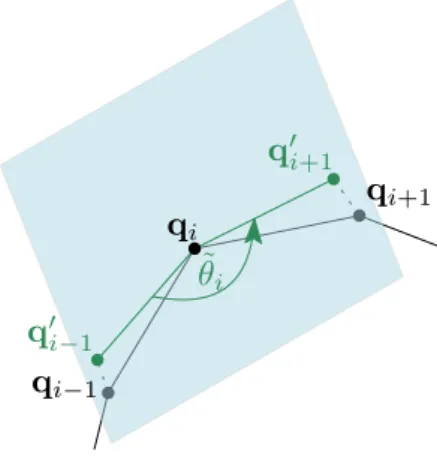
By forming the sum of the (squared) rotation angles between successive edges of this planar polyline, an approximation of its (squared) geodesic curvature integral is effectively obtained [Crane and Wardetzky, 2017]:. In the subsequent phases of the algorithm, label candidates will be merged and removed with the aim of arriving at one of the allowed label configurations. Decisions about which labels to merge or remove will be based on the properties of the real or virtual vertices defined by pairs of candidate labels.
The estimated angle is formed at the center of the transverse, as shown in Figure 4.5a. A virtual angle is classified concave if the normal lies transversely in the opposite direction of one of the endpoint tangents. Even if the angle is classified strongly convex based on these criteria, the surface that fills the region between the label candidates and the angle can be geometrically complex (e.g. with high Gaussian curvature), as in the case of the bottom angle in figure 4.5. B.
Multi-sided parametric surfaces over curved domains
- Introduction
- Previous work
- Non-uniform parameterizations
- Multi-sided surfaces
- Concave and multiply connected patches
- Domain generation
- Local parameterizations and harmonic interpolation
- Curved Domain Bézier patches
- Surface definition
- Split boundaries
- Discussion and case studies
- Summary
In contrast, the ribbons of a Concave GB patch, or a CD patch, are completely independent. dive: each may have a different pair of degrees, and even when the degrees are the same, the control point positions may differ, see e.g. the green-red and red-blue angles in Figure 5.5b. The previous methods are described for B-splines with open knot vectors – the problem of interpolation of boundary conditions, the use of clamped knot vectors is not elaborated. This represents a solution to an important problem, using modified (cubic and quintic) mixing functions in the cross direction, extending that of the convex GB patch [Várady et al.,2016].
In these contexts, the boundary curves are often assumed to have special properties, such as being major curvilinear lines – the methods in this work do not make such assumptions about the ribbons. This section presents the basics of the CD Bézier patch definition - further details are found in the paper [Várady et al.,2020]. The content of this chapter is based on parts of the publication [Várady et al.,2020].

Generalized B-Splines
- Introduction
- Surface equations
- Rational terms
- Editing the interior
- Discussion and case studies
- Convex vs. curved domains
- A complex vertex blend
- Polyhedral design
- Multi-sided patches at extraordinary vertices
- Multiply-connected surfaces
- Sheet metal parts
- Special cases
- Summary
The internal tape matches the surface of the label and a GBS patch blends seamlessly with the bottle tapes. Pij,k refers to the jth control point in the kth row, which is multiplied by a product of the basis function of the corresponding B row Njdi,ξi and the degree 2mi+ 1 BernsteinBk2mi+1 polynomial. Then, the patch is defined over the domain Ω, with global parameters (u, v), as a sum over the bars:. 6.3) GBS patches are thus very similar to CD Bézier patches - the main differences are in the use of B-spline basis functions along the boundary, the choice of rational terms and also in the local parameterization, which will be discussed in section 7.2. 2.
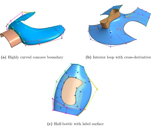
The control points of the ribbons ensure that the boundary constraints are satisfied, but the interior is created indirectly by an algebraic combination of the basis functions. If the fullness of the patch is not sufficient, or further shape adjustments are required, internal control points should be added. The cross derivatives for the perimeter ribbons and the hole loop must both be orthogonal to the plane of symmetry of the bottle, so that the two halves can be joined together smoothly.
Generating curved domains and their local parameterization
Curved domain generation
- Tangent development
- Closing the loop
- Interior loops
- Osculating development
In the next subsection, a method for determining the contracted polynomial is described, which remains a faithful approximation of the original form. Expressed in terms of node positions, this could be formulated as a hard nonlinear, nonconvex optimization problem. The solution to this problem is simply to change the size of the original angles:. b) Geodetic leveling, before closure (c) Geodetic leveling, after closure.
Then, the positions of the nodes must be changed minimally to close the loop, which could be formulated as a form optimization problem. If this problem were to arise, the adaptation of the method described in [Salvi and Várady, 2018, sec. The resulting smoothed binormal frame can be used to develop a polyline in a manner that is faithful to the external shape of the curve.
Local parameterization
- Local parameterization for CD Bézier patches
- Local parameterization for GBS patches
- Periodic interior loops
- Improved h-coordinates
- Implementation notes
- Surface evaluation
Remember that each side is composed of several segments, corresponding to the nodal spans of the B-spline bands. 7.9) where =si orhi, and bf codes for the aforementioned Dirichlet boundary conditions for the limited subset of the boundary Df ⊂∂Ω. Compare the overlapping multi-loop parameterization of the previous section shown in Figure 7.7c with the new periodic scheme shown in Figure 7.7f.
This is generally not satisfied by harmonic functions, so - with inspiration from [Crane et al., 2013] - the gradient vectors of the original h-coordinate are first normalized, then a least-squares fit to this vector field, calculate. The positive effect on the parametric deformation of the final patch can be observed by comparing Figure 7.9a and Figure 7.9b. Note that this discretization should not be considered part of the definition of CD Bézier or GBS patches.
Summary
Sparse direct solvers are very efficient for typical problem sizes in the current setting; the implementation used the Eigen library [Guennebaud et al., 2010]. The CD Bézier and GBS surfaces presented in the dissertation were evaluated at the vertices of a triangle of their parametric domains, simply by substituting in the patch equations. Differential quantities, such as normal vectors, or curvatures were approximated based on the 3D triangle mesh in the usual way [Botsch et al., 2010].
The domain generation algorithm and harmonic local parameterizations are well defined in transfinite settings, and meshless methods such as Monte Carlo integration [ Sawhney and Crane , 2020 ] could be used to evaluate curved domain patches (or even their derivatives). to any precision.
Thesis summary
This thesis is based on Section 3.2 of this thesis, and has been published in the journal publication [Vaitkus and Várady,2018b] and the conference paper [Vaitkus and Várady, 2018a]. This thesis is based on Chapter 4 of this thesis, and was published in the journal publication [Vaitkus and Várady, 2019]. This thesis is based on Chapter 5 of this thesis, and was published in the journal publication [Várady et al.,2020].
This thesis is based on section 7.1 of this dissertation and was published in a journal publication [Várady et al., 2020]. This thesis is based on section 7.2 of this dissertation and was published in a journal publication [Vaitkus et al., 2020].1. This thesis is based on Chapter 6 of this dissertation and was published in a journal publication [Vaitkus et al., 2020].1.
Conclusions and future work
Conclusions
Future work
The quality of the mesh extension was found to be adequate for practical purposes, but further improvements are possible, e.g. CD Bézier and especially GBS corrections have proven to be very practical multi-site representations, but of course many problems remain for future research. The domain generation and local parameterization have been found to be reliable in practice, but there is still some room for improvement.
For example, combining the tangent and osculating variants of the domain generation algorithm in an adaptive way is an interesting problem to be solved. In general, the quality of a versatile patch is determined by a complex interplay of the ribbons, the domain shape and the local parametrizations – considering each aspect simultaneously also proves to be a challenging research project. Neither the harmonic local parameterization nor the patch definition requires that the domain be a subset of the plane, only that it be a two-dimensional manifold (with boundary) that can be discretized in e.g.
Acknowledgements
Bibliography
In Proceedings of the 23rd Annual Conference on Computer Graphics and Interactive Techniques, pages 313–324. In Proceedings of the 12th Conference of the Hungarian Society for Image Processing and Pattern Recognition (submitted). In Proceedings of the International Conference on Mathematical Methods for Curves and Surfaces II, pages 501–527.
Appendix
Formulae
- Gradient and Jacobian
- Mass matrix and polyharmonic systems
- ARAP energy smoothness
- Symmetric ARAP distortion
The polyharmonic energies of the form (3.15) of the partially linear function f (of the vector x, y or the coordinates of the vertex) are then discretized as quadratic forms. The smoothness of the ARAP partial-linear mapping distortion measure is measured by energy. The distortion of parametric surfaces can be quantified as the deviation of the domain-to-surface mapping from local isometry.