History of Gr¨obner bases and combinatorial applications
Introduction to the theory
We shall see that it is not so simple, but still we will be able to give an upper bound for |G|. For zero-dimensional vanishing ideals I(V), the Buchberger-M¨oller algorithm [12] provides a fast way to obtain a Gr¨obner basis and the standard monomials in one go.
Main results and structure of the thesis
- Monomials and term orders
- Standard and leading monomials
- The existence of Gr¨obner bases
- Reduction
- The reduced Gr¨obner basis
- The Hilbert function
We shall see that this happens because G is not a Gr¨obner basis for the ideal hGi. But when ˆf reduces with respect to a Gr¨obner basis of I, then it is a linear combination of standard monomials of I, and so ˆf ∈ I if and only if fˆ= 0.
Zero dimensional ideals
Algebraic multisets
Due to some misuse of notation, instead of Pw we will use the latter - even if the characteristic is not zero and w. Properties of Pw known from differential operators (such as Leibniz's rule) become clearer in this way.
Primary decomposition
We call y∈Fn a point of I (or a point associated with I) as Qy 6=F[x] in the primary decomposition of I. We now prove an easy characterization of Gr¨obner bases of vanishing ideals of finite multiple sets.
Alon’s Combinatorial Nullstellensatz and a conjecture of R´edei 31
One could think of the rank as the effective number of variables of the polynomial. For a fixed ideal, we somehow get a set of monomials Stan(I) as a result of the game.
The multiset case
Since F is finite, we have only finitely many conditions that a polynomial can satisfy.
Points in almost general position
Vanishing ideals of the plane
Let gv be in I and lm (gv) = svt`v, so by the induction hypothesis we know that t`v divides gv. There exists a monomvt`+`v−`w ingw(s, t)·t`v−`w which cannot be canceled by the reduction because `+`v−`w < `v but every monomial of gv. Thus, with the maximum value of v, we have v =v0 and sosvt`0 ∈Lm (I), which contradicts the definition.
The game for almost general points
THE LEX GAME 46 The next claim (and its proof as well) is similar, except that we have to apply Corollary 4.3.3 in the proof, which was not at all trivial to verify. In fact, the reason Stan monomials are generally not equal to standard monomials is that the straightforward generalization of these statements is not true (see Example 4.4.1). Suppose that I1 and I2 are zero-dimensional partition ideals such that their points all have the same final coordinates, but they are distinguishable by their second-to-last coordinate (i.e., if y is a point of I1 and z is a point of I2 , then yn =zn and yn−1 6=zn−1).
Without loss of generality, we can assume that the common last coordinate of the points I1 and I2 is 0, since the change of variables x0n = xn−yn does not affect the standard monomials. In particular, if n = 2, then the standard and Stanov monomials are the same for every zero splitting ideal. In the first round, Lea guesses, since this is the only possible last coordinate of points Iy.
We have just seen that the latter corresponds to exwexmn−1xwnn ∈ Lm (Iy,y0), which is not the case since m < my,y0.
The general case
Computing the Stan monomials
- Standard monomials of a trie
- The naive approach
- Another try
- Running time
Our goal is to construct U such that the set of vectors corresponding to leaves of U is the set of exponent vectors of Sm (T). The following example gives the result of the algorithm applied to T = T(V) of the set V of Figure 4.1. As we will prove shortly, the three U that we end up getting through the algorithm are the three of the exponent vectors of Sm (T(V)).
The trie U given by the above algorithm are the trie of exponential vectors Sm (T). Here we will study some direct consequences of the Lex game for vanishing ideals of finite multisets V. The standard monomials of the primary components of two corresponding ideals are the same.
The second part of the consequence concerning (non-multi-) setsV ⊆ {0,1}n has been proved in [5] by a different method.
Generalization of the fundamental theorem of symmetric poly-
For the second statement, let F be any field and think of G as a subset of F[x]. GAME APPLICATIONS - WARM UP 60 is a symmetric polynomial, then it can be uniquely written as a finite sum. For the set of points V defined above, xw is a lexicographic standard monomial I(V) if and only if w is n−1).
On the other hand, if, for example, wi ≥i, then Lea can in (n−i+ 1) steps select all the elements in {z1,. But the leading monomials of the fi for all term orders ≺ considered in the theorem are the same, thus Smlex(I(V)) ⊇ Sm≺(I(V)). Due to the equality of the cardinalities of the two sides, we have that the standard monomials are the same for all term orders considered.
An application of the fundamental theorem of symmetric polynomials, together with Sm (I(V)) = {xw : w n−1)} gives the existence of the required form for f.
Hilbert function and inclusion matrices
APPLICATIONS OF THE GAME – A WARM-UP 63 instead of I(VF) for the vanishing ideal of VF. Note that VF ⊆ {0,1}n, and so, when playing Lex (VF;w), we will assume that Stan always chooses yi from {0,1}, even if both numbers were among Lea's guesses and so Stan loses the game by such a choice. Theorem 2.1.20 implies that among all multilinear monomials of degree at most m, the maximum number modulo I(F) of linearly independent monomials is the same as the number of standard monomials of I(F) of degree at most m, that is HF(m).
Since F[x]/I(VF) is isomorphic to the space of functions on VF, it is also isomorphic to F|F|. APPLICATIONS OF THE GAME – A WARM-UP 64 To complete the proof, note that xM(vF) equals 1 if and only if M ⊆F, and it is zero otherwise. Let PF,m be the linear space of functions from VF to F that can be represented as homogeneous multilinear polynomials of degree m.
Incidence matrices and their rank are also important in the study of finite geometries.
Wilson’s rank formula
Lexicographic standard monomials
Theorem 6.1.3 is valid for all ideals of the form I(F), where F is any family such that for all f ∈Zeither ¡[n]. If w= 1 then Stan wins if and only if|FD−t,1|= 2, since Lea can only check one of the two possibilities. Now the description of the standard lexicographical monomials of a modulo q complete `-wide family is as follows.
Proposition 6.1.3 suffices to show that the network path criteria from the theorem hold if and only if 0 ∈ D(w). It is clear from Theorem 6.1.4 that every multilinear leading monomxM satisfies conditions (1) and (2) of the corollary. If this is true, then conditions (1) and (2) of the corollary together with Theorem 6.1.4 imply that xM is a leading monomial.
Obviously x2i −xi ∈ I(F) for all i ∈ [n], so we only need to check if x2i are minimal generators of the initial ideal.
A Gr¨obner basis
On the other hand, ˆg(vF) is exactly the sum of the coefficients of the monomialsxF0. The set of variables of this part and of the one we have already considered are disjoint, so we will no longer need reduction withx2j−xj. Therefore, we can use the fact that the largest term of a product is the product of the leading monomial, and it is therefore sufficient to show that the leading term of Qt.
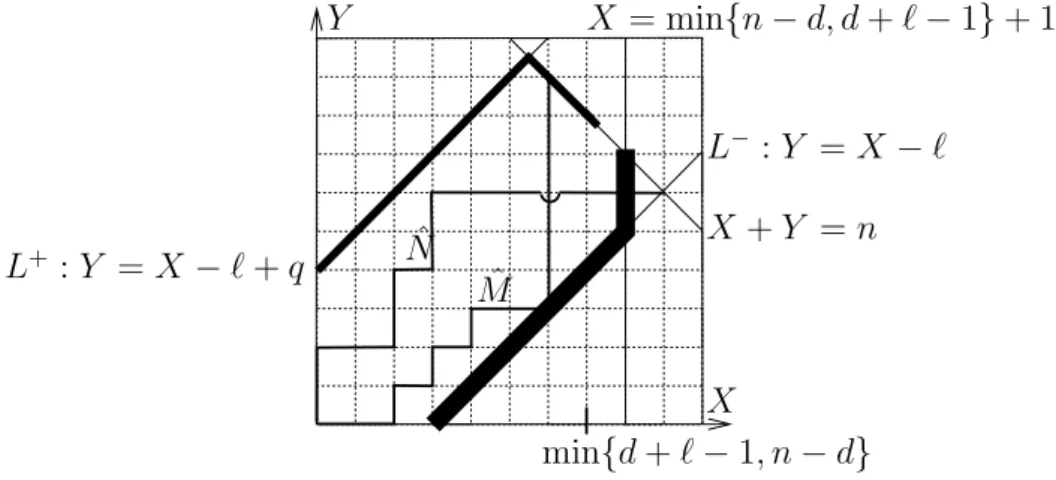
Using the rule for leading product monomials again, it suffices to verify that mi < ut−i. In this case, we must also take into account that the leading monomial is from n−d+1Q. xmi−1) is the product of the leading terms of xmi−1, i.e. xmt+1. To this end, we show that ˆN goes above and to the left of ˆM, or – to be more precise – we show that the X coordinate of the intersection of ˆN and X+Y =j is less than or equal to the X coordinate of the intersection of ˆM and X+Y =j for all j ∈[n].
Here we used that the leading monomial xM has the highest degree in our polynomials.
The Hilbert function
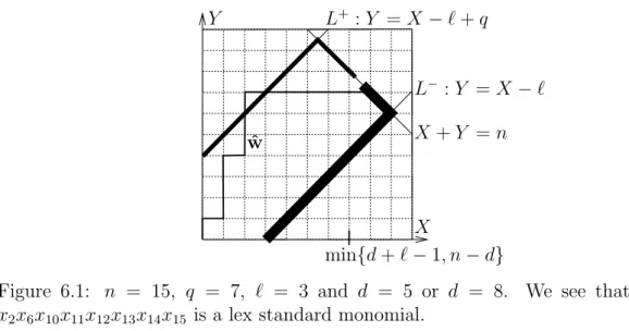
We denote by C the set of those lattice paths that connect the origin to the point P without reaching either of the two lines L+ and L−. Our final set of lattice paths D to examine consists of all paths from the origin to P that fail to reach L− before reaching L+ (it cannot reach either). Instead of writing only C and D, in this proof we again indicate their dependence on the end point (nX, nY) of the lattice paths, while leaving F out of the subscript of HF.
Therefore, if m ≤ r then the set of lattice paths corresponding to standard monomials of degree at most m is. The number of standard monomials of degree nX between r0+ 1 and dhem is given by the lattice paths. The corresponding lattice paths have the property that they do not reach L− before touching L+ and that they end with (nX, n−nX) for some nX ≤m, that is, they all belong to the set.
In the proof (equation (6.11)), we have seen that the right-hand side is exactly the number of such lattice trajectories.
Maximal cardinality of L-avoiding L-intersecting families
Then we write fG for the polynomial in Fp[x] that we obtain from ˆfG by reducing its integer coefficients modulo p.
Families that do not shatter large sets
This gives Sm (I(G)) ⊆ Sm (I(F)), so we can bound the cardinality of the standard monomiles of G by the number of standard monomiles of F of degree at most m. BuildSmTrie(T) of T builds the trie U encoding the standard monomials of V SmListFromTrie(U) the list of standard monomials of the trie U. 34;PURPOSE: Given V a finite set of points (ie integer vectors of the same length) it computes the lexicographic standard monomials of the vanishing.
THEORY: See the article at http://www.math.bme.hu/~fbalint/pub.html/lexgame.pdf. ASSUMPTANCE: V is a list of intvecs of the same length. A node can have a reference to its parent, a list of references to its children, a value (that is, the integer on the edge between the node and its parent), a reference to a node on the same level of the trie, and references to two of the leaves that are descendants of the node. 34; PURPOSE: Creates the trie that encodes the standard lexicographical monomials of the points associated with the trie argument.
Winkler(editors), Gr¨obner Bases and Applications, London Mathematical Society Series, Volume Proc of the international conference "33 Years of Gr¨obner Bases".