Graph Coloring with Local and Global Constraints

Minimizing the sum of the coloring and minimizing the number of colors can be very different. Ordinary edge coloring is NP-hard [Hol81, LG83], but can be solved in polynomial time for bipartite graphs.

List edge coloring planar graphs

Planar bipartite graphs

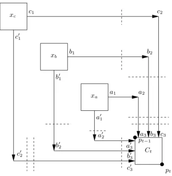
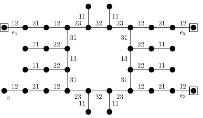
The three numbers in each frame show the three colors assigned to the edge in the three possible colors of the graph. Make a copy of variable setting gadgetGx for each variable x and a satisfaction testing gadget GC for each section C of the formula.

Outerplanar graphs

By [JS97], list coloring can be solved in O(|V|k+2) time if the treewidth of the graph is at most k. Given a formula φ in conjunctive normal form with n variables and m clauses, we construct an example of the list edge coloring problem in such a way that the graph can be colored if and only if φ is satisfiable.

Figure 2.3: The reduction from 1-in-3 SAT to the list edge coloring problem. We connect the variable setting components and the satisfaction-testing components with pairs of edges.

List multicoloring of trees

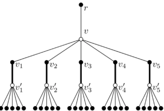
The construction will ensure that the colors given in the central node correspond to an independent set in G. On the other hand, if there is an independent set of size kingG, then we can assign these colors and extend the coloring to the nodes : oseui,1 orui,2 is not contained in the independent set, so tovi can be assigned.

Graphs with few cycles

A polynomial case

For every simple graph G, list edge polycoloring with demand on the vertices can be solved in polynomial time. The list edge multicolor problem can be solved in polynomial time for trees and odd.

Figure 2.6: The list edge multicoloring with x(e) ≡ 2 has no solution, but with y(v) ≡ 4 there is a coloring valid for the vertices.

Graphs with few cycles

Since every coloring valid for the edges is also valid for the vertices, the list edge multicolor problem has a solution if and only if there is a coloring valid for the vertices that satisfies the requirements in Lemma 2.3.8. If there is a perfect matching M in G such that|Fi∩M|=ki for every 0≤i≤, then construct a coloring Ψ valid for the vertices, as in the proof of Theorem 2.3.4.

Applications and extensions

In Section 3.4, we strengthen this result by showing that the problem remains NP-complete for planar 3-regular bipartite graphs. For interval graphs already 2-PrExtis NP-complete [BHT92], but 1-PrExt can be solved in polynomial time [BHT92].

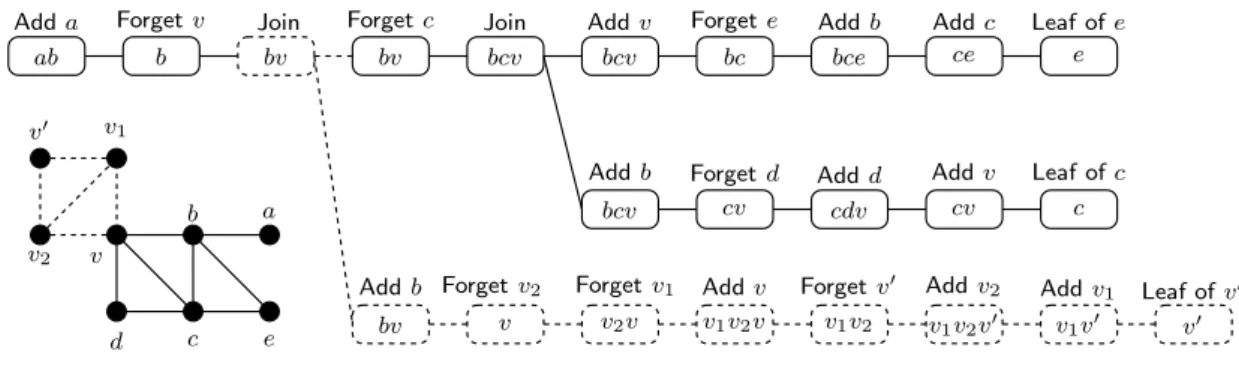
Figure 2.8: (a) The edges of the path correspond to the two-day jobs. (b) The pendant edges represent one-day jobs

Tree decomposition

It is easy to see that by splitting the nodes of the tree in an appropriate way, we can convert the tree decomposition of G into a nice tree decomposition in polynomial time. Clearly, this modification results in a nice decomposition of the tree, and if we perform it for each previously colored node v, then we obtain a decomposition of G.

System of extensions

Change the coloring of ψ1: change the colors of C\C1 such that ψ1(v) =ψ2(v) holds for every v∈S2 (this can be done because K is a clique, so both ψ1 and ψ2 assign different colors to nodes in S2). Again, permute the colors of C\C1 in the coloring of ψ1 such that ψ1 assigns to K\S exactly the color in C.

The algorithm

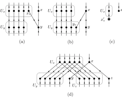
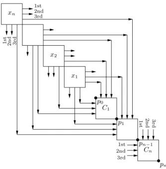
For every u ∈ S, in current fy, there is one unit of current consumed by the terminal at yu. The current consumed at node y and z is directed tox to the arc −yx,→ −zx, respectively.

Figure 3.3: Construction of the network when node x is of the following types: (a) add node for v ∈ W , (b) forget node for v (either in W or not), (c) leaf node for v ∈ W , (d) join node.

Matroidal systems

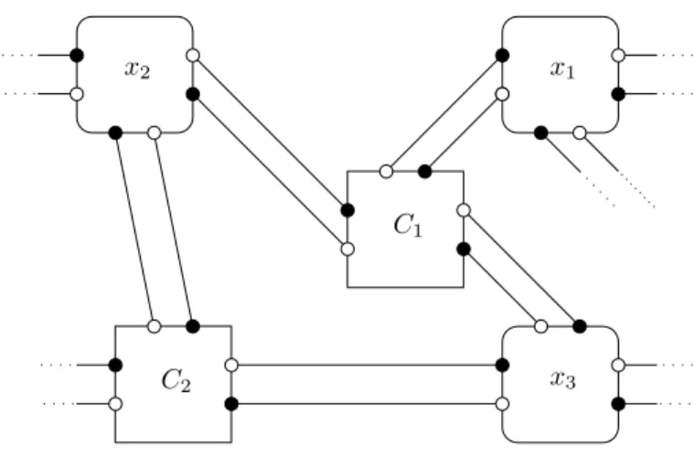
However, based on the feasible flow of networkNr, one can construct a precoloring extension of the graph. We have seen that the feasible flow of network Nx represents a set Sx ∈ S(Gx, Kx).

Figure 3.4: A non-chordal graph G and a clique K = { v 5 , v 6 , v 7 } such that S (G, K) is not the projection of a matroid (|C| = 4).

Applications

By observation 3.1.6, the number of sources iNxis corresponds to r=|Cx|, so that every possible flow of Nx corresponds to an−→. By Lemma 3.1.7, ifS ∈S(G, Kx), then there is a possible flow in Nx, where flow is only consumed by the terminals of Ux that correspond to the elements in S.

The Eulerian disjoint paths problem

The reduction

Assume that there are no bad crossings to the left and above the vertex −1. The destination for demandsαi and βi is in the clause component corresponding to the clause for the current instance of the variable.

Unit interval graphs

The reduction

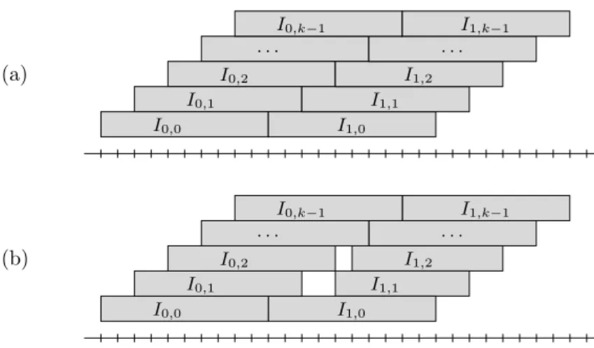
On the other hand, assume there is proper precoloring scope with mcolors. Color each edge,j of the lattice graph with the color assigned to the corresponding intervalIi,j.

Figure 3.10: (a) In every k-coloring c of the (open) intervals, I 0 ,i and I 1 ,i receive the same color for 0 ≤ i ≤ k − 1 (b) In every k-coloring c of the intervals, c(I 0 ,i ) = c(I 1 ,i ) for i = 1, 2 and either c(I 0 , 1 ) = c(I 1 , 1 ), c(I 0 , 2 ) =

Complexity of edge precoloring extension

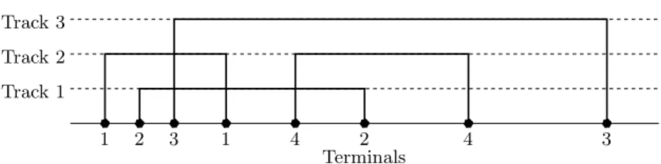
Therefore, minimizing the total length of the wire is equivalent to minimizing the amount of coloring in an interval graph. Minimizing the coloring error is clearly equivalent to minimizing the amount of coloring. Deciding whether G has a zero-error coloring is a special case of the minimum sum edge coloring problem.

Bipartite graphs

Planar graphs

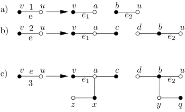
Thus, the error of Si is at least 3 and can only be 3 if the overhanging edge is colored with color 1. The error on the internal vertices is at least 6 in any color: there are at least 3 errors in each of S1. However, the error is strictly greater than this: at least one of e1 and e2 is colored with a color.

Figure 4.3: Each precolored edge is replaced by the corresponding subgraph on the right.

Approximability

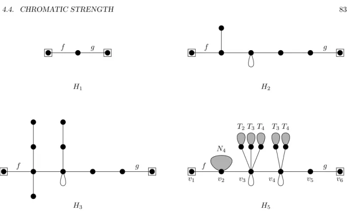
If a coloring has zero error on the internal vertices of the tool variable, then it colors all three edges of the pendant with color 1. If a coloring has zero error on the internal vertices of the tool, then clearly f andg has color 1 or 2. On the other hand, if both f and g have color 1, there is at least one error in the internal vertices of the device.

Partial 2-trees

In every coloring of G, the error is at least K(1) on the inner vertices of the 4 connected trees. In each coloring, the error is at least K(2) on the interior corners of the variable setting gadgets. In each coloring, the error is at least K(3) on the inner vertices of dem/2 copies of A8n−1.

Chromatic strength

Vertex strength of bipartite graphs

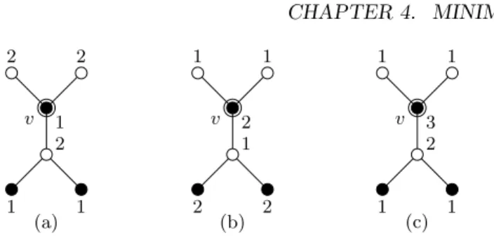
Precoloring extension (PrExt) is a generalization of vertex coloring (see chapter 3): we get a graph G(V, E) with a subsetW ⊆V of vertices with a preassigned color, the question is whether this precoloring can be extended to a proper k- coloring the graphene. In I4, the sum of the coloring decreases if we use the colors shown in frames. In everyVv, depending on the color ofv, the coloring can be extended to one of the three colorings shown in Figure 4.12.

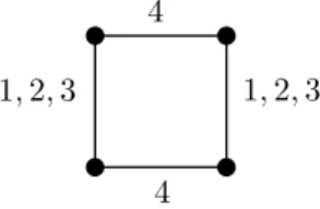
Figure 4.12: The new vertices attached to vertex v of H, and three minimum sum colorings that assign to vertex v (a) color 1, (b) color 2, (c) color 3.

If fi (1≤i≤k) in each k-edge coloring of G denotes the number of hanging edges of color i, then fi has the same parity as n. For each graph, it was first checked whether it is 3-edge colorable, and if so, the sum of the best 3-edge coloring and the best 4-edge coloring was determined by a simple backtracking method. Unfortunately, we cannot provide hand-verifiable evidence that this sum cannot be achieved by a 3-edge coloring.

The complexity class Θ p 2

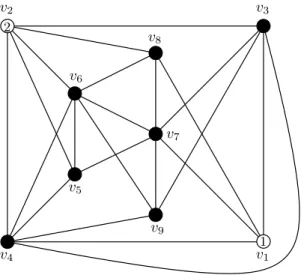
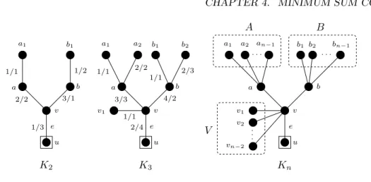
Furthermore, even if ϕi is not satisfied, Gih has the largest independent set sizeni+mi−1 that does not contain a vertex (an assignment satisfying every clause except Ci,1 yields such an independent set). That is, every maximal independent set G induces a maximal independent set for every partition class. We claim that every largest independent set G contains ˆv:=b1 if and only if|{wi:wi ∈A}|is odd.

Figure 4.15: A graph with Δ(G) = χ (G) = 3 but s (G) = 4. The ﬁgure shows a minimum sum edge coloring with sum 29 using 4 colors, every 3-edge-coloring has sum at least 30.

The reduction

On the other hand, if both and have color 1, there is at least one error on the internal vertices of the gadget. Asv ∈D, then color gadgetSv using coloringψ∗: each pendant edge has color 2 and there is 1 error on the internal vertices. Asv∈D, then we use coloringψ of the vertex apparatus: every pendant edge of Sv has color 1 and there is no error on the internal vertices.

Special vertex gadget

Furthermore, in Section 5.3 we show that although minimum sum edge coloring is polynomial-time solvable for trees [GK00, Sal03], the multicolor version is NP-hard even if every claim is 1 or 2. In Section 5.4 we give a polynomial time approximation scheme (PTAS) for minimum sum edge polycoloring of trees. We show that there is a minimum sum polycoloring with at most O(logp) privileges at each vertex.

Figure 4.19: The graph H 1 , H 2 , H 3 , and H 5 .

Preliminaries

Operations

There is no conflict on the right, since the completion time of v+ 1 is less than . The completion time of n decreases by fΨ(n)−x(n), so the total increase in sum is at most β+x(n)−fΨ(n). This requires at most left fixed β, and increases the completion time of n−1 by at most fΨ(n)−fΨ(n−1).

Figure 5.1: Parity shift from u to v in the range a to b. a) Before the operation. b) After the operation;

Bounding the reduced sequence

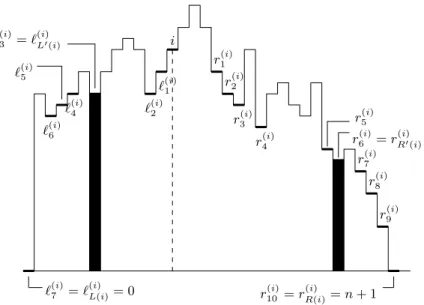
If d1+d2+d3 is "large", then this means that the finishing times in the left sequence decrease rapidly, what should we show. Let be the number of left steps in the reduced left sequence and denote by (si1), (si2), . sim) subsequence containing all steps up of the reduced left sequence. Using the following lemma, we can bound the number of local minima in the left-reduced sequence using the bound on the number of steps in the right-reduced sequence.

Figure 5.3: The left and right sequence of the node i.

Optimum coloring

If we can prove that in the truncated case of Ψ, the sumL(i) +R(i) is strictly smaller than in Ψ, then according to the induction hypotheses there is an optimum color Φj of the truncated case where Φj(i) has less as L(i) +R(i) privileges. It is easy to see that the reduced left (resp. right) sequence of nodei in the truncated instance is the prefix of the reduced left (resp. right) sequence in Ψ. In the case described above, [1,2C] is clearly a left critical set for node 1, since if α-colors in this set are missing in a color Φ, then fΦ(1) ≥2C+α.

Perfect graphs

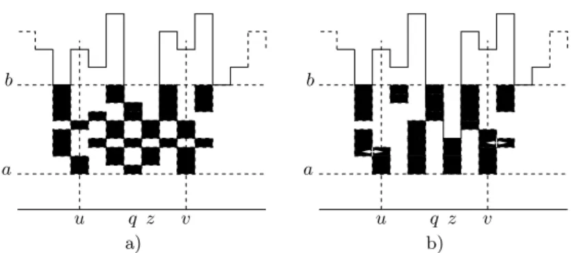
NUMBER OF CONDITIONS 101 First, we introduce a well-studied coloring problem, where the number of different colors used must be minimized instead of the total sum. It can be easily verified that the integer solutions of the dual program correspond to the solutions of the makespan problem: we select some independent sets, possibly selecting a set several times, so that every vertex in at least x(v) selected independent sets are . If no vertex has end time between a and b, then we can rearrange the colors between a and b without increasing the end time of any of the vertices.

Complexity of minimum sum multicoloring for trees

The penalty gadgets

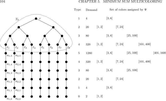
It is easy to prove that the completion time of a node of tipitiisfΨ(v) =g(i) +g(i−1) =x(i) +x(i−1) since it will have exactlyg(i−1 ) colors "passed" and the completion time of type nodes is greater than the completion time. If fΦ(Pi)≤fΨ(Pi) and Φ are different from Ψ, then there exists av∈Pi such that fΦ(v)< fΨ(v), so it is not empty. Since H is nonempty, there is at least one subgroup Sv in the partition with fΦ(Sv) > fΨ(Sv), in contradiction.

Figure 5.7: The tree T t,d,C for t = 2, d = 4 and C = 6. The nodes on the same level have the same type.

The reduction

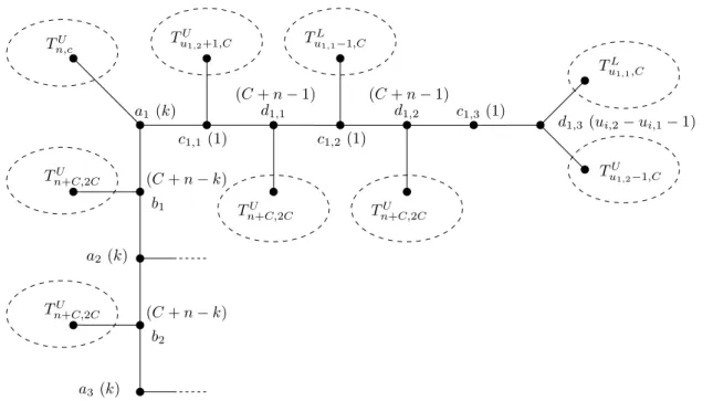
Therefore, the coloring Ψ is an optimal coloring and the tree satisfies the requirements of the proposal. The trees attached to these nodes ensure that this color must be either ui,1 or rui,2, one of the end nodes of an edge in G. Also note that u≥ui,1, sinceci,2 cannot use the colors below ui , 1: these colors are assigned to the root of the attached TuL tree.

Figure 5.8: The tree T for m = 3. For the sake of clarity, the nodes c i,j , d i,j for i ≥ 2 and the subtrees connected to these nodes are omitted

Complexity of minimum sum edge multicoloring for trees

It can be easily verified that this is a good A-coloring (ie optimal) and edgerv can have any of the colors b, c. To prove the other direction, given a satisfying assignment, we construct an A-well coloring of the tree. Get a good coloring of the subtreeT4j corresponding to variableblinxj so that its root edge uses the colors {4j+ 1,4j+ 2} (ie

Figure 5.9: The tree T 6 . The strong edges have demand 2.

Approximating minimum sum multicoloring on the edges of trees

Preliminaries
Scaling and rounding
Bounded demand
Bounded degree
The general case

The number of edges in the tree is O(n), so the total running time of the algorithm is Moreover, it can be easily verified that the total end time of the edges inFv can be expressed asfΨ3(Fv). The other parts of the algorithm can be done linearly in time in the size of the input.

Figure 5.11: Partitioning the tree into high-degree stars (shaded regions) and low-degree components (D = 4).

Complexity of clique coloring

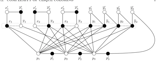
It can be verified that the coloring defined above correctly colors every flat edge of the graph. First suppose that K is colored white, then it contains some of the 2n vertices xi, xi (1≤i≤n), and at most one of the vertices p (1 ≤≤q) (the vertices ternsyj, yj are black). First suppose that there is a (k+ 1)-clique coloring ψofG, we show that it induces ak-clique coloring of G.

Figure 6.2: The construction for the formula ϕ = (x 1 ∧ x 2 ∧ y 2 ) ∨ (x 1 ∧ x 3 ∧ y 2 ) ∨ (x 1 ∧ x 2 ∧ y 1 )

Clique choosability

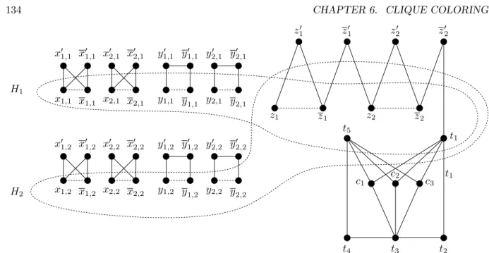
To prove the other direction, we show that if ∃x∀y∃zϕ(x,y,z) does not hold, then for each list assignment there is the correct clique coloring. If there is a coloring of this path such that t1 and t5 have a different color, then this can be extended to a proper vertex coloring of the kernel of G. Since the coloring is a proper vertex coloring of the kernel of G, it is sufficient to check maximum cliques greater than 2.

Figure 6.4: The structure of graph G in the proof of Theorem 6.3.1 for n = 2, m = 2, p = 2, q = 3.

Hereditary clique coloring

This coloring can be extended to Gin so that the straight edges are colored correctly (ie it can be extended to the inside vertices of the copier and edge tools). It turns out that we can formulate the problem as coloring a chord graph. A graph is out-of-plane if it can be embedded in the plane such that every vertex is on the outer infinite face.

Figure 6.5: The γ-copier Z 1 . Figure (a) shows the graph Z 1 that served as base for constructing Z 1

Approximation algorithms

As in the case of minimization problems, the smaller α, the better the algorithm. Our goal is to find an arrangement of cities such that the total distance between cities is minimized. The PTAS for the Euclidean TSP can be generalized to the d-dimensional version of the problem for any fixed d.

Oracles and the polynomial hierarchy

This follows quite easily from the NP-completeness of the Hamiltonian cycle problem (see e.g., [Pap94]). In Proceedings of the West Coast Conference on Combinatorics, Graph Theory and Computing (Humboldt State Univ., Arcata, Calif., 1979), pages 125–157, Winnipeg, Man., 1980. In Proceedings of the 3rd Hungarian-Japanese Symposium Mathematics discrete and its applications, pages 164–.