Parts of current PhD research work were developed in the framework of the project. At this step, it is also reasonable to exclude from the model graph those junctions where these subnetworks intersect other parts of the modeled network.
Relevant methodology
This iteration continues until the last part of the trip request is delivered to the network. The relative gap for the entire network is the degree of difference between an assumed ideal state (equilibrium) and the actual state of the network.
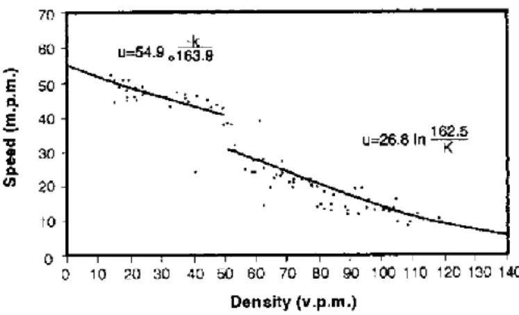
Traffic flow characteristics
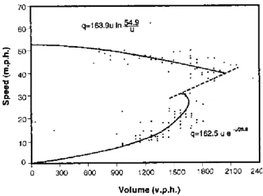
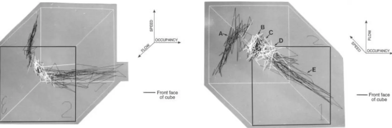
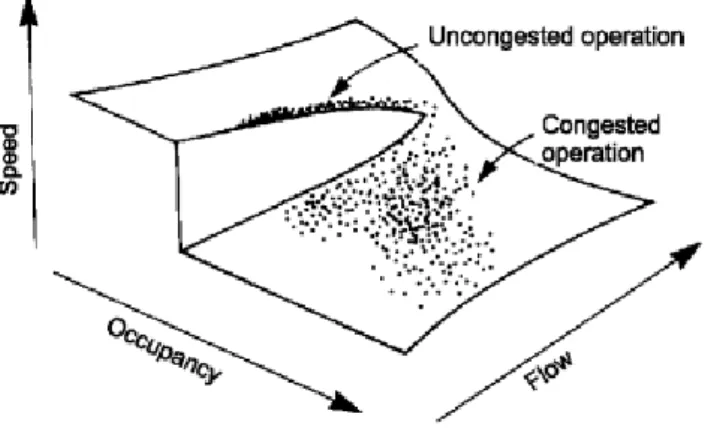
The later approach, using the principles of catastrophe theory, is much more promising. The performance of the Catastrophe Theory model was compared with other traffic flow models (Acha-Daza & Hall, A Graphical Comparison of the Predictions for Speed Given by Catastrophe Theory and Some Classic Models, 1993) (Acha-Daza & Hall, The Applicarion of Catastrophe Theory to Traffic Flow Variables, 1994) and found it to be better than the classical approach.
Volume-delay functions
Rahmi Akcelik (Akcelik, 1991) developed this particular delay function when trying to deal with shortcomings of the Davidson variant (Cascetta, 2009) of the delay function. The specialty is the exact opposite of the previous Vatzek function: the function allows over-allocation more than usual.

Microsimulation
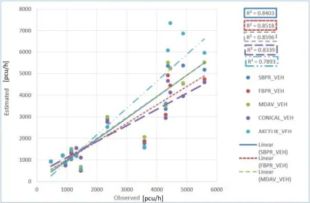
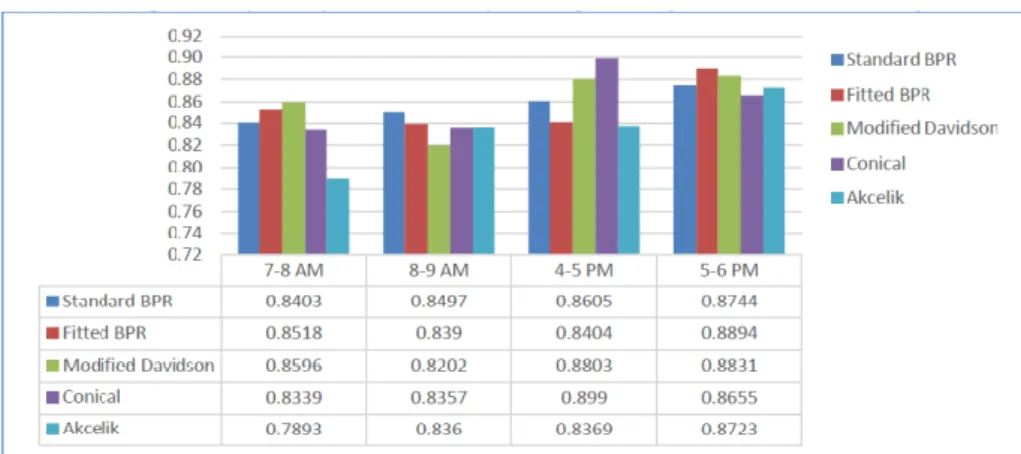
A study in Washington (Milone & Moran, 2010) compared the goodness of fit of Conic and Akcelik functions and concluded that although the Akcelik function fit slightly better than the Conic, they advised the use of Conic functions due to their better convergence rate.
Conclusion
This fact highlights the importance of delay functions in transport modeling and also points out that due to the high number of iterations, the computation of any new type of time delay must be efficient to provide a viable alternative to existing methods. For this reason the dissertation focuses on solving the specific time delays of the junctions in the same way as they are defined at a link level to be able to incorporate the observed effects in the existing volume delay functions, eliminating the need for a new implementation.
Introduction
Methodology
The directional distribution of vehicle flows is also constant: 20% of the turning volume in the larger flow and the same proportion of turning volumes in the smaller flow. In the case of a four-pronged intersection, the number of vehicles crossing in the smaller flow is 40% (30-30% remains for turning right and left).
Autonomous data acquisition
To produce different results, it is necessary to modify the value of the 'random seed' variable. Some features of the model are easily modified through the VISSIM Component Object Model (COM) interface (PTV AG, 2012b).
Results
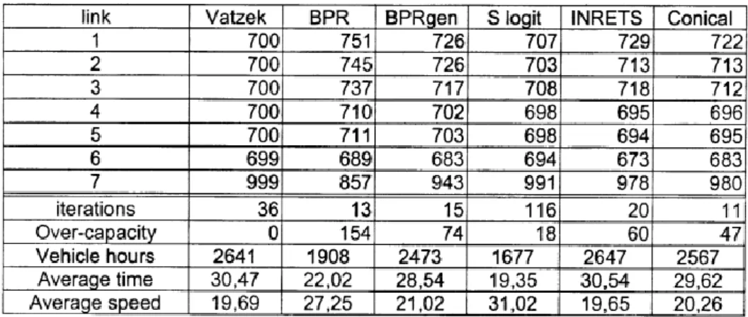
The function parameters determined – using equation (3-1) – are listed for the reduced set in Table 7 below.

Conclusion
Thesis I
Introduction
Temporal range
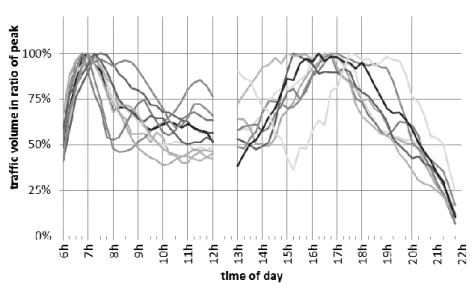
To determine the average length of the peak, its rising and falling characteristics, traffic flow data was analyzed from a series of measurements. It is obvious that the period of maximum value can be divided into three phases, which confirms the assumptions. As for the overloaded state, its most important characteristic is the sustained peak length.
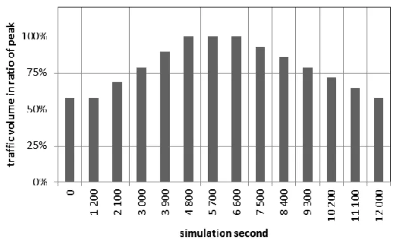
Peak values were normalized individually, so for each location and measurement 100% means the actual maximum flow (e.g. at measurement 2 at site 3 the peak flow of 713 pcu/h corresponds to 100%, but at measurement 4 of the same site 100% value expressing 788 pcu/h traffic flow). According to these values, the length of the peak period was set to 45 minutes, with a 60-minute long ascent and a 75-minute long falling phase for a total length of 3 hours. The start and end volume values are 58% of peak volume (see vehicle volume input defined for microsimulation on Figure 23).
Spatial extents
Modeling considerations
Given the length of the simulation models, a warm-up period of 1200 seconds has been included in the simulation. Upstream and downstream parts of the network had to be extended by 'rolling up' the links to the extent (see Figure 24) implied by the 'unwinding' transformation of the resulting spatial vehicle records. Traffic flow characteristics can be measured point by point by defining data collection points at different distances along the network and collecting attributes of passing vehicles over time.
Note that the results displayed on Figure 25 and Figure 26 are from early tests, which are spatially flawed, as the model was not large enough to contain all the congestion. Limits of the congested network can be derived directly from the inspection of various transient characteristics. Considering the length of the networks, vehicles had to drive for a maximum of 20 minutes to approach the intersection, so results from 0 to 1200 seconds were discarded.
Results
Dividing the records into time slices makes them more understandable and also allows the observation of congestion dynamics: a temporally arranged set of visualized instantaneous velocity graphs shows the fluctuation of the congestion limit and its dissipation in time - again at the level of current theories (Figure 27) ). The span of these intervals was set to 5 minutes (300 seconds) for practical considerations: the amount of vehicle records over the 40 km length of the investigated network was still manageable, while the number of intervals remains synoptic. It is important to note the bipolar nature of three-legged intersections: during high traffic volumes, the main flow with a left turn suffers a significant amount of delay with increasing vehicle queues, while the opposite main flow (with a right turn) can be relatively undisturbed.
Analogies
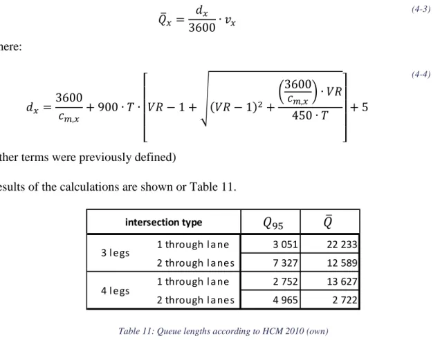
Calculation of queue lengths for the two value pairs gives the result 162 and 60 metres. In the Highway Capacity Manual (HCM) (Transportation Research Board, 2000 and 2010), service levels are categorized by control delay, from LOS-A to LOS-F, parallel to the Hungarian standard (its categorization was partly derived from the HCM). Although the control type of the method does not correspond to the control type of the simulation models (which is two-way yield), it is reasonable to compare fixed queue lengths with the simulation results, since the flows studied in the current calculation are left turns of the main flow, which are also not required to stop before yielding in TWSC junction.
However, the 95th percentile queue length does not account for the effects of a congested left lane, where the waiting vehicles block the through lane. That is why it is also useful to calculate average traffic jam lengths on the basis of average delay times, whereby the risk of lane blocking does have an effect. The average queue length is the product of the average delay per vehicle and the flow rate:. other terms were previously defined).
Conclusion
Further uses
Thesis II
Introduction
Framework
Each model intersection had a separate left turn lane on the main road and no turn lanes on the secondary road. VII Each approach to the main road has only two directions at three-arm intersections: either 'left and through' or. IX The notation concept is: nxmL, where n='number of intersections', and m='number of node legs' (i.e. 3 or 4).

Function fitting
Initial values for variable 𝜀 parameter vector x must be specified at the start of the algorithm. Return values (results) of the algorithm are the refined parameter vector x, and the sum of least squares g to be able to assess convergence. First, the behavior of the model function was analyzed by using a fixed value for each parameter (also for the variable t), changing a single parameter, and recording the change in the function value.
This property prevents convergenceXI of the minimum search algorithm, therefore the formula had to be modified. The NLLSM described above requires the construction of a Jacobian matrix of the partial derivatives of the model function (see equation (5-11)). Although Figure 37 suggests that the iteration should have been stopped at the 50th cycle, since there is very little change in the value of the norm at later steps, a closer examination of the delay function curve response through the iteration shows otherwise.

Analysis
Using the non-linear least squares method (NLLSM) specified earlier (chapter 5.3) the delay function parameters were estimated. Taking a look at the graphs of the functions in Figure 42, it is clear without further calculation that a VDF could not be reproduced by simply scaling one of the other curves. Dividing the junction chain function values by the single junction function values shows an almost linear relationship up to the point where traffic volumes exceed the capacity of the model configuration in one of the compared functions.
This confirmation of the hypothesis leads to another study: a similar study of the inverse functions. The conspicuous large difference at higher traffic volumes could be considered less significant as it is on the 'model' part of the curve where measured data had little or no influence on the shape of the function. However, the use of the VDF from the singular junction model propagates the inaccuracy of the fit at lower volumes to other junction chains.

Conclusion
Further uses
Thesis III.a
Thesis III.b
Scaling the function variable unifies the VDF formula for homogeneous crossing series for each intersection type. VDFs are fundamental components of the network modeling procedure, determined by evaluating traffic flow measurements. Another set of experiments confirmed the viability of microsimulations to create different yet distinguishable datasets of traffic flow measurements, supporting further research studies.
Using this property, it was possible to formulate a single junction-specific VDF that reduced the effort involved in applying the set functions during later use. These methods have been developed with a generic approach and can be used in other research scenarios in the future – not limited to the extensions of the current project. These parameters can also be integrated with the results of the current research to create highly detailed junction-specific volume delay functions.
Thesis I
Thesis II
Thesis III.a
Thesis III.b
Sub Main(sender As Object, e As System.ComponentModel.DoWorkEventArgs) Dim worker As BackgroundWorker = CType(sender, BackgroundWorker) Dim oXL As Excel.Application. Dim oTC As TrafficComposition Dim oInp As VehicleInput Dim oInps As VehicleInputs Dim i As Integer. Dim dVols kot nov seznam (of Double) Dim lVols kot nov seznam (of Double(,)) Dim currVols(,) kot celo število.
Sub ChartXL(ByRef oSheet As Excel.Worksheet, ByRef aliRng As Excel.Range) Dim oChart As Excel.Chart. Dim xMax As Double = 0 Dim yMax As Double = 0 Dim oRng2 Kot Excel.Range Dim oCell As Excel.Range oRng2 = oRng.Columns(1) Za vsako oCell v oRng2.Cells. Osi (Excel.XlAxisType.xlCategory).crossesat = 0 .Axes(Excel.XlAxisType.xlCategory).minimumscale = 0 .Axes(Excel.XlAxisType.xlCategory).maximumscale = xMax .Axes(Excel.XlAxisType.xlCategory).mino runit = 50 .Axes(Excel.XlAxisType.xlCategory).majorunit = 250 .Axes(Excel.XlAxisType.xlCategory).minortickmark.
Axes(Excel.XlAxisType.xlValue) 1. Sub PutXL(ByRef oSheet As Excel.Worksheet, ByVal sData() As String, ByVal nRow As Integer, Valgfri congested As Boolean = False).