Irreversible thermodynamical study of elastic, thermal expansion, rheological and heat conduction processes in

Furthermore, the modeling and simulation of the rheology of solids gain a new potential application area for the design of gravitational wave detectors. I would like to thank the staff of the Department of Energy Engineering for the pleasant atmosphere in which I worked.

Figure I.1: Snapshots about the temperature distribution of a polymeric sample, taken by thermal camera during a uniaxial rupture test [1]

Motivation

From the exotic behavior of superfluids to engineering applications of beyond-

This last type of heat conduction also differs strongly from Fourier heat conduction (see figure I.3). It is now clear that several challenges and promises lie ahead for non-Fourier heat conduction engineering.

Figure I.2: Left: A simplified schematic picture about Peshkov’s experiment [2]. In a glass tube (G), heat pulse signals are generated by the heater (H), and temperature is measured by the thermometer (T)

How does rheology of solids contribute to design of gravitational wave detectors? 6

1 The term thermodynamics comes from the Greek words therme (heat) and dynamis (power). As a consequence of the previous statements, the Gibbs relation on the specific entropy can be derived.

Figure I.8: Characteristic strain – frequency diagram of different gravitational wave sources and sensi- sensi-tivity of different gravitational wave detectors [34].

Solids in the small-strain regime

3(trε)1, εd =ε−εs, (II.27) where d ands denote the deviator and spherical parts of the tensors, respectively, and 1 is the identity tensor. The deviator and spherical parts are isotropic independent [tr(AdBs) = 0 for each A,B] so (II.26) can be given as.

Internal Variable Methodology

More general quadratic expansions can also be applied, but such expansions can result in nonlinear expressions, so here we restrict ourselves to the simplest form given by (II.29). By substituting the expression (II.33) into the entropy balance, other, unusual terms are generated in the entropy production rate density.

The GENERIC framework

The effect of thermal expansion on heat conduction

Edεd+Es[εs−α(T −T0)1], (III.2) where Ed and E are the deviatoric and spherical elasticity coefficients1, respectively, and α is the coefficient of linear thermal expansion. EsαT0∇ ·v=λ∆T −%cε∂tT, (III.10) which, together with the balance of linear momentum (II.21) (with volumetric force density neglected). From the equality of (III.12) and (III.13) a non-Fourier-like heat conduction equation on temperature is obtained, i.e.

In other words, the lhs of (III.14) makes a contribution to the rhs through a dimensionless factor τ`22.

Parameter testing

Since the specific entropy of the Duhamel-Neumann material depends only on the spherical part of the stress and the deviatoric part of the stress (thus also the inverse relation, i.e. the deviatoric part of the stress) does not depend on the temperature (see equations (III.2) and (III.5)), the above expression can be given as self-explanatory. From the measurable coefficients of the material given in table III.1 through the formulas given before, the dimensionless characteristic coefficients are presented in table III.2. The "effective" thermal diffusivity is shifted by a few percent, compared to the "constant strain" thermal diffusivity, at room temperature.

Therefore, the deviation from Fourier heat conduction measured in room temperature heat-pulse experiments cannot be explained by thermal expansion.

An interpretation of entropy current multipliers via GENERIC

Systematic generalization of heat conduction beyond the Fourier theory

One-dimensional state space
Two-dimensional state space
Three-dimensional state space
Generalized ballistic-conductive heat conduction reduced from a four-

Comparing (III.25) with (III.22), the usual entropy flux density jS = T1jE and the entropy production rate density. The entropy production rate density (III.55) is given only in these variables, i.e. the dissipation potential ΞJ. Consequently, instead of this assumption, let us return to equations (III.53) and identify the heat flux density with the entropy conjugate internal variable as .

The first term on the right-hand side (III.108) represents the reversible contribution, while the second term is the irreversible contribution of time evolution.

A short comparison of IVM and GENERIC

Conclusions

The heat current density is often identified with an internal vector variable, however, we have shown that, from a general theoretical point of view, identifying the heat current density with the conjugate of the internal vector variable is more favorable. The introduction of antisymmetric irreversible coupling terms in the symplectic (ie reversible and entropy-conserving) part of the equations, which increases the numerical possibilities. Since the extended entropy balance [based on (II.24)] must be of the form.

It is important to note that the antisymmetric part of the coefficient matrix does not contribute to entropy production.

Internal variable rheology of solids realized in the GENERIC formulation

Temperature as state variable

Temperature has the same relation to specific entropy as seen in section IV.2, now used in the opposite direction (ie, what is a variable and what is a function): The thermodynamic consistency condition d˜dTs0 = T1 d˜edTermal which comes from the Gibbs relation [and which is the manifestation of (IV] the third equation.4). Moreover, since (IV.46) does not contain nonlocal (gradient) terms, we can perform the transformation directly in the form. 7 The results (IV.52), (IV.53) can also be derived directly from the time evolution formula and the degeneracy conditions.

Indeed, by substituting (IV.43) into (IV.10) and rewriting it in terms of temperature, the evolution equation for T is obtained, and it turns out to coincide with the fourth row of M˜ δδ˜Sx˜, so the whole evolution equation is preserved under the transformation.

Conclusions

Numerical proof of the total power-saving property of the scheme for a three-dimensional Cartesian grid. The continuum system that is the subject of the study is important in itself - it is the PTZ rheological model for solids. As a simple analysis of the PTZ model, for "slow" processes, understandable with respect to the time scales.

At the same time, the dissipative nature of the PTZ model requires the minimal possible amount of dissipation error to reliably describe the decrease of wave amplitudes.

Figure V.1: Dimensionless rear-side velocity history in dimensionless time for dimensionless pulse length 0.2 calculated by Backward Differentiation Formula

The numerical scheme in one spatial dimension

Stability

The Hooke case
Poynting–Thomson–Zener case

The stability of the corresponding physical model, the Poynting-Thomson-Zener body, is ensured by the second law of thermodynamics. Nevertheless, a criterion of one of these two methods need not directly be a criterion of the other method. 3According to Jury [148], a matrix is internally positive if the determinant of the matrix and all its internal elements are positive.

Interiors only come into the picture from ≥3, so in our case only positive definiteness of the matrices themselves needs to be ensured.

Numerical results and investigation of dissipation and dispersion errors

Hookean wave propagation
Poynting–Thomson–Zener Wave Propagation

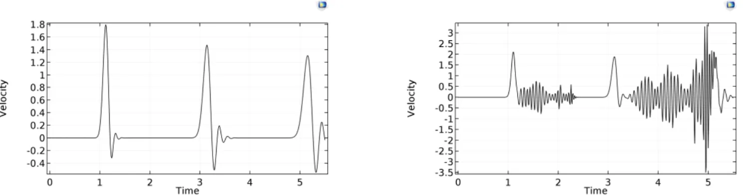
Although the run time is highly dependent on other factors, it provides a good picture to compare the effectiveness of the commercial approach and the scheme presented above. The physical explanation of the signal shape (Figures V.9-V.10) is that the fastest modes propagate with speedcˆ(recall Section 2), transporting the front of the signal, while slow modes travel with c <ˆc, gradually falling behind and forming, little by little, a thicker tail. In parallel, the space-time picture shows that this tail effect is less relevant than the overall reduction of the signal due to dissipation.

Regarding the energy results, the remarkable fact is that all ingredients v, ε, σ, T are computed via discretized time integration, so total energy savings are not built in, but are a test of the quality of the whole numerical approximation.

Figure V.6: Wavy dispersion error and decrease by dissipative error for the Hooke system when C = 1/2, with N = 100.

The numerical scheme on a three spatial dimensional Cartesian grid

Numerical solutions and the role of total energy

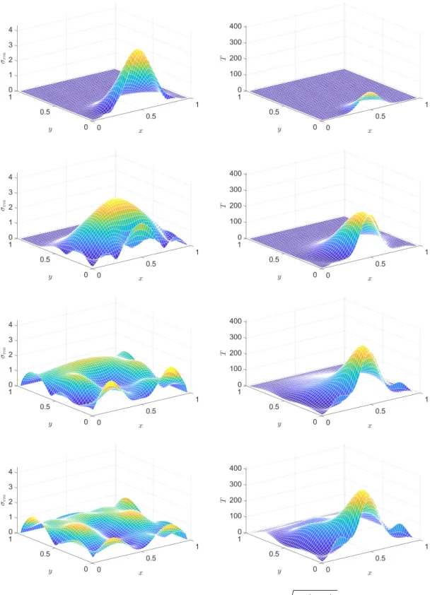
The example on which the scheme is demonstrated is a long square cross-section beam, which is thus treated as a plane stress problem. Simulation results for Hooke elastic material can be found in [48], the scheme was found to provide satisfactory and reliable solutions, which is almost trivial since the scheme is a second order generalization of the symplectic Euler method. The scheme presented here also functions satisfactorily on this point, as shown in figure V.19.

For energy, we perform summation, over the integer-centered discrete cells, of the energy terms discretized along the above lines, including averaging as for (V.93) where necessary, also in the time direction (for kinetic energy).

Figure V.17: Snapshots of the distribution of the stress invariant r

Discussion

Equations of elasticity and rheology in the force-equilibrial approximation

Equations (VI.1), (VI.2) and (VI.5) form a closed system of equations with respect to elasticity, which together with the appropriate boundary conditions can be solved. When dealing with the rheological problem, equations (VI.1), (VI.2) and (VI.6) form a closed system of equations. Since the constitutive equation (VI.6) contains time derivatives, in addition to the boundary conditions (which may in general be time-dependent), initial conditions are also required to solve the problem.

When dealing with the rheological generalization of the problem described above, in addition to (VI.1), (VI.2), (VI.6) and boundary conditions (which may in general be time-dependent), initial conditions are required to ensure the uniqueness of the solution, since the constitutive equations contain time derivatives [see (VI.7) and (VI.8)].

Preparations

In this case, all equations and boundary conditions must be satisfied at all instants of time. In the rheological case, all fields are functions of time and space, and all equations and boundary conditions must be satisfied for all time instants. In general, when more than one boundary condition is nonzero in a problem, then the problem can be divided into such subproblems in which only one boundary condition is nonzero.

For modeling the process of drilling or loading/unloading pipes or tanks, this function can be simply chosen as . VI.15).

The method of four elastic spatial pattern sets

This elastic stress solution with the corresponding strain-dimensionalized stress solution satisfies equations (VI.12), (VI.16) and the boundary conditions for each admissible. From Hooke's law, the deviatoric and spherical parts of the stress can be given by these as. VI.36). All that remains is to derive relations between the unknown coefficient functions ϕm(t), ψn(t) based on (VI.18).

Substituting these matrices into the deviatoric and spherical parts of (VI.41) and (VI.42), then from «(VI.18) Eqs.

Figure VI.1: Outline, coordinate systems and notation for the considered problem.

Practical applications

Finally, the displacement field - displacement understood with respect to the primary initial state of the continuum - can be calculated via Cesàro's formula (VI.4), i.e., . VI.55) Here we note that the rigid-body-like freedom of movement and rotation must be fixed3. The upper right corner illustrates the evolution over time of the move field for a fast opening (movements are magnified for visibility), while the second and third rows show the time evolution of the coefficient functions for slow (left column), medium speed (middle column), and fast (right column) openings. The observable non-trivial time dependencies resemble those for the anisotropic problem (see Figure VI.4).

Demonstrating the applicability of the method to general linear rheological models, Figure VI.8 presents the time evolution of the coefficient functions with respect to the Kluitenberg–Verhás – Hooke model, i.e., σd=ηζd+ (E1d/Es) ˙ζd+ (E2d/Es) =ζζd. VI.58) For simplicity, the coefficient of σ˙dis is chosen to be zero, so the inertia index (see [43]) is necessarily positive, so, accordingly, rheological (damped) oscillations will be present.

Figure VI.3: Cylindrical bore opened in an infinite, homogeneous and isotropic stress field

Conclusions

The numerical dispersive errors can be eliminated if α = 12 and the value of the Courant rheological number Cˆ = qE. Farkas, "Application of the modified law of heat conduction and equation of state to dynamical problems of thermoelasticity", Periodica Polytechnica Mechanical Engineering, vol. Liu, “Method of Lagrange Multipliers for Exploitation of the Entropy Principle,” Archive for Rational Mechanics and Analysis, vol.

Maxwell, "On the Dynamical Theory of Gases," Philosophical Transactions of the Royal Society of London, vol.