This paper compares the limited commitment risk sharing model, with and without preference heterogeneity, to the benchmarks of perfect risk sharing and autarky. The scope to introduce preference heterogeneity in the case of perfect risk sharing has been explored by several papers. More precisely, we model changes in each household's consumption relative to the average consumption in the community.
Estimation of the perfect risk-sharing model, as well as the autarky standard, are relatively straightforward. Therefore, we compare the limited commitment risk-sharing model with a certain precision with other risk-sharing models.2 Vuong's (1989) tests are appropriate in this context, see Fernández-Villaverde, Rubio-Ramírez and Santos (2006). Both the heterogeneity of preferences and the constraints on the implementation of risk-sharing contracts turn out to be important.
Perfect risk sharing
Think of the explanatory variables in the utility function as mean deviations from their community in the following, abusing the record.5. The next three subsections detail how the full risk-sharing (subsection 3.1), autarky (3.2), and limited-commitment risk-sharing (3.3) models are estimated. We do not assume that the model is correctly specified, and we do not compute the variance-covariance matrix of the estimated parameters without the assumption that the equality of the information matrix holds.
Both the first and second derivatives of the log-likelihood function can be calculated analytically here.
Autarky
Risk sharing with limited commitment
First, let's focus on the individual effects η and assume that we know the realization of the measurement error in the consumption of household i at time t−1, denoted by εji,t−1, drawn from the distribution εi,t−1, N( 0, γ2). In the case of complete risk sharing, the predicted spending distribution was independent of δ, the discount factor. Remember that εji,t−1 denotes the realization of the measurement error in the consumption of household i at time t−1.
To deal with the fact that measurement error enters the state variable update, we first write the probability. Average income can be thought of as a proxy for the household's income-generating capacity. For the rest of the community, quantiles are calculated above the mean income in the community.
We consider seven income statements for each household, and four for the rest of the community. The estimation of the limited-stakes risk-sharing model includes both simulation and approximation. The calculation time is approximately proportional to the number of income states, where we take 7×4 = 28, and the square of the number of grid points onxi.
Increasing the number of grid points would be helpful in better approximating the real solution of the model. In this article we do not assume that any of the models are correctly specified, and it is possible that in the case of limited-stakes risk sharing, a larger number of grid points would lead to a decrease in the model's fit to the data.
Model selection
Additional approximation error may come from the fact that we limit the number of iterations when solving the model. In a recent paper, Ackerberg, Geweke, and Hahn (2008) argue that, in terms of the asymptotic properties of the maximum likelihood estimator, the approximation error in computed dynamic models has similar effects with a limited number of simulations. They provide Monte Carlo evidence that the method does indeed work, assuming the estimated model is correct.
As a robustness check, we examine below whether our results are affected if the number of grid points is changed. If the two models are not nested, then under the null hypothesis the two models are equally close to the true model. If the two models are nested, and we want to account for the possibility that the unconstrained model is not specified correctly, then below null.
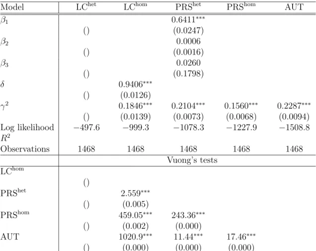
We compare five models: complete risk sharing with heterogeneous preferences (PRShet), complete risk sharing with homogeneous preferences (PRShom), autarky (AUT), limited commitment risk sharing with heterogeneous preferences (LChet) and limited commitment risk sharing with homogeneous preferences ( LChom). Alternatively, assuming that consumption growth is measured with error, as for example in Cochrane (1991), the errors of the first differenced equations are i.i.d. Pakistan's Punjab has well-developed factor and product markets compared to the poor semi-arid areas on which much of the risk-sharing work in developing countries is based (Kurosaki and Fafchamps, 2002).
Furthermore, consumption data was collected from the female head of the household, while income data was collected from the male head. The assumption that the measurement error in consumption is independent of the income measure is therefore more compelling than usual.
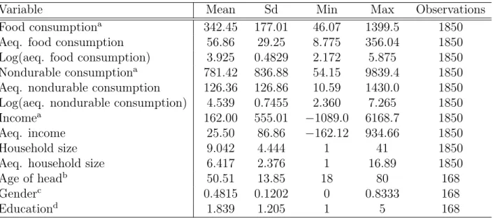
Variables used
We consider three variables when specifying preference heterogeneity, namely the age of the household head at time 1 (age), gender, and education. The heads of households in the sample are almost exclusively men. We therefore construct a measure of the gender composition of households. To measure educational level, a categorical variable is used, based on the final educational performance of the head of the household.
In particular, education is equal to 1 if the head is illiterate, 2 if he has attended primary school or learned to read, 3 or 4 if he has attended secondary or high school (including technical studies), respectively, and 5 if he has go to college or university. We delete the observation if consumption is missing, income is missing, or any component of income is outside a reasonable bound. We delete households whose household head is over 80 years old, or if the household head changes during the three-year interview period.
11Wealth is the sum of the values of land, houses, other assets (such as television sets, watches), tools and livestock. Measured income is only a fraction of measured consumption, reflecting general under-reporting and the fact that agricultural production was severely affected by poor weather conditions in the years of the survey. For the structural estimates, we remove the 5% extreme consumption and income observations from the pooled panel.
Finally, total income should be equal to total consumption in society, since savings have been assumed away. To achieve this, the income is rescaled so that the total income is equal to the total consumption at each t.
Existing evidence
On the other hand, Ogaki and Zhang (2001) are unable to reject perfect risk sharing for the vast majority of villages examined, when relative risk aversion is not constant. The authors argue that previous tests of perfect risk sharing do not take into account the possibility of reduced relative risk aversion. The current paper allows risk aversion to depend on more observables and compares the perfect risk-sharing model with a well-defined alternative, namely the limited-commitment risk-sharing model.
First, note that if the relative risk aversion coefficient is higher, it means that the marginal utility of consumption is lower, given that consumption is greater than 1. Exceptions include the seminal work of Binswanger (1980), who finds no difference in aversion risk between men and women. Evidence on the effect of age and education on risk aversion is mixed.12 If we think of education as a proxy for wealth, we can discuss the sign of β1 based on how risk propensity should vary with wealth.
There is agreement in the literature that absolute risk aversion decreases as one becomes richer. 12Guiso and Paiella (2008) find that risk aversion is independent of wealth and disease with education, based on the willingness to pay for a hypothetical risky security. On the other hand, Palsson (1996) finds that relative risk aversion increases with age, based on data on the portfolio decisions of Swedish households.
Based on insurance data, Halek and Eisenhauer (2001) find a positive relationship between education and risk aversion. In Holt and Laury's (2002) laboratory experiment on choosing between risky options, risk aversion is independent of age and education.
Main results
In the second panel, the p-values from Vuong's tests are in parentheses, indicating whether the model of the line can be rejected because it is as close to the actual generation process as the model of the column. Tables 2 and 3 show that the coefficient of relative risk aversion is positively related to education, our measure of wealth. This result is consistent with the hypothesis of Arrow (1965) and Pratt (1964) that relative risk aversion increases as wealth increases.
Age and gender do not significantly affect σi, but the gender coefficient has the expected positive sign.
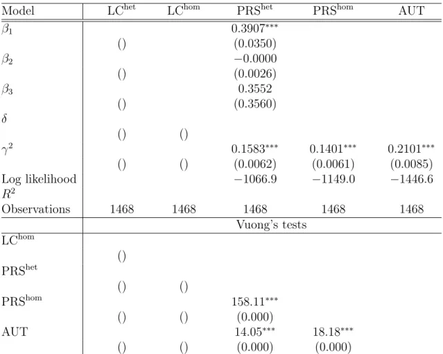
Robustness checks
The measurement error in income is assumed to be multiplicative and lognormally distributed.
Perfect risk sharing
Autarky
Risk sharing with limited commitment
Given household characteristics and an acknowledgment of the preference shock today, the enforcement constraint can be written in a recursive form as First, given the distribution from which income is drawn, the measurement error does not affect the optimal intervals characterizing the constrained efficient risk-sharing contract, as the model is solved using a grid of income. Second, the introduction of measurement error in income can plague the nonparametric estimation of the income process.
We could perturb the observed income and then recalculate the model against the measurement error plot matrix. Again, simulation is a simple way to solve this problem and the model solution does not need to be recomputed, so the computation time is only moderately increased. This would allow policy makers and NGO members to better understand the effects of their programs.
First, other models of risk sharing could be incorporated into the analysis, such as the private information risk sharing model (Wang, 1995). Comments on "Convergence properties of the likelihood of computed dynamic models" by Fernández-Villaverde, Rubio-Ramírez and Santos. This appendix describes how the limited commitment risk sharing model is solved numerically.
The first task is to solve the optimal intervals that characterize the model's solution. The support of the grid is the series of relationships between marginal utilities of households k and i given the income and consumption observations. Unfortunately, the algorithm does not converge from an initial guess for the value functions, but the value of the perfect risk sharing case will.14.
Note that the two enforcement restrictions cannot bind at the same time because only one of the two households can be requested to make a positive net transfer.