market dynamics: A statistical physics approach

The individual behavior of the units is associated with the overall behavior of the system. Another feature related to the latter may be non-stationarity, i.e. system dynamics change over time.

Trading mechanism

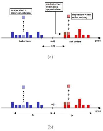
Since the number of orders varies, the reconciliation between orders is not necessarily one-to-one. If the volume of the starting order is less than the volume at the opposite best price, then the best price does not move.

Figure 2.1: Example of a limit order book. Snapshot taken from inetats.com

Financial correlations

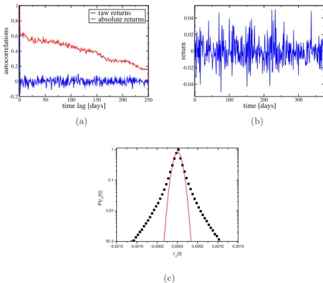
Autocorrelation functions of daily returns and daily absolute returns for the stock price of Exxon Mobil Corp. XOM) for the period January 2007 to June 2008.; (b). Logarithmic daily returns for the stock price of Exxon Mobil Corp. XOM) for the period January 2007 to June 2008.;.

Stylized facts and universality

This empirical fact is very closely related to the slow decay of absolute correlations, but we prefer to mention it separately due to the fact that it can be related to bursts of trading activity by market participants. An interesting question is to what extent these stylized facts are due to the behavior of traders and what is the role of market rules and mechanisms in creating them.

The Efficient Market Hypothesis

In practice, the classical taxonomy of the information sets distinguishes between three forms of market efficiency [Fam70]. In the following, we will review some of the shortcomings of the hypothesis and examples of ineffectiveness.

The role of humans: Behavioural finance

We see that the set of information is central to the definition of EMH, and the information that traders use plays a central role in financial research. Prospect theory, one of the most important ideas in behavioral finance was developed by two psychologists, Kahneman and Tversky, in 1979 [KT79].

Figure 2.4: A hypothetical value function in prospect theory. Figure taken from [KT79].

Modeling

Phenomenological models

In fact, most of the models later derived to model time series rely on some kind of random walk. With his approach, Bachelier predicted several results from the second half of the twentieth century.

Multi-agent models

This is actually the case for the logarithmic price evolution of an asset over time. In such a market there is certainly no need to model traders' preferences and decisions separately, since they are all rational in the same way.

Experiments

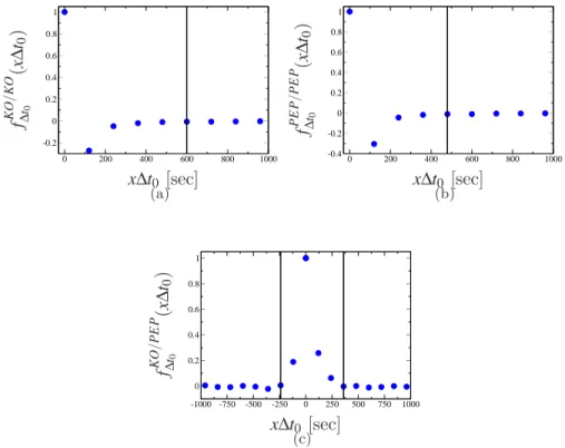
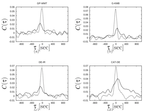
We study the correlation between the changes in the position of the two random walkers. The noise level of the calculations is also included in the plot (straight lines).

Time evolution of correlations

Lagged correlations

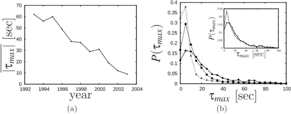
The distributions that reach more and more sharply near zero show the reduction of the time shifts. The inset shows the same distribution for the years 1993 (circles) and 2000 (triangles); we can see that the tails of the two distributions are similar, indicating strong deviations from the overall trend.

Figure 4.1: Example plots showing the changes in the correlation functions for the years 1993 (solid) and 2003 (dashed).: (a) GP/WMT pair; (b) G/KMB pair;

Equal time correlations

Conclusions

Later, even in the case of equal time correlation coefficients, we will see that the year 2000 is an exit year, probably due to the dotcom crash. The development we found is a sign of the changing collective behavior of market participants, which is the result of a change in the mechanism, not the will of the individual [TK06].

A new approach to the Epps effect

Empirical observations
Decomposition of the cross-correlations
Model calculations
Fitting to the data
Conclusions

5−10 does not lead to a measurable reduction in the characteristic time of the Epps effect (where the characteristic time is defined as the time scale for which the cross-correlation reaches the degree 1−e−1 of its asymptotic value). 4.5) Using this relationship, we can write the time average of the product of returns on a large time scale (∆t) in terms of averages on a short time scale (∆t0) as follows:.

Figure 4.4: The cross-correlation coefficient as a function of sampling time scale for the period 1993–2003 for the Coca-Cola Pepsi pair

Efficient estimator of correlations

The method

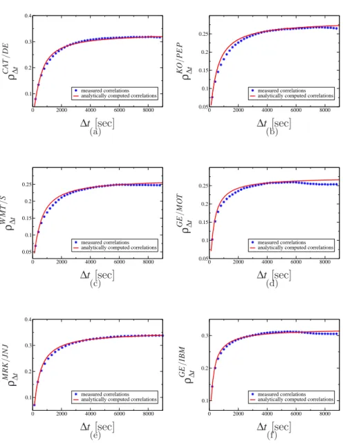
Assuming ∆t=n∆t0 with n a positive integer, we can derive the generalization of Equation 4.12 in the following form:. By plugging these quantities into Equation (4.35) with ∆t>>∆t0, we get a good estimate for the correlation coefficient as a function of ∆t. We use correlated random walks and show that in the case of directly measuring the correlations in large time windows we need very long time series to have a good estimate for correlations.

Demonstration

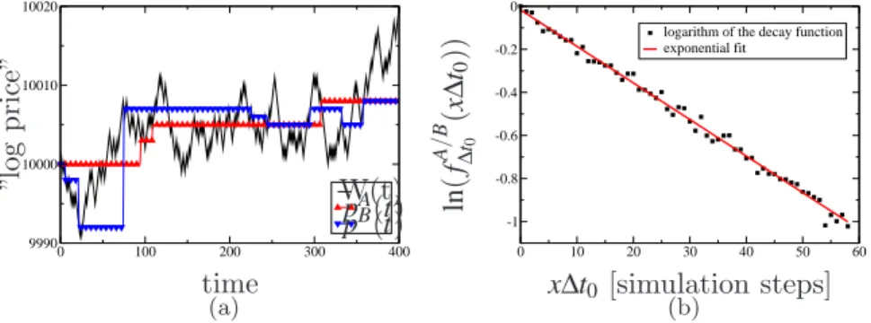
In blue we show the mean and standard deviation of the direct measurements calculated over the ensemble of 50 time series pairs. The circles show the correlations determined using the decomposition method, and the (red) curve is the piecewise cubic Hermite interpolation of the correlation values. The same improvement is obtained for the precision of the extrapolated asymptotic correlation coefficients.

Figure 4.10: (a) Comparison of the directly measured correlation coefficients and the coefficients determined through the decomposition method in case of exponen-tially distributed sampling intervals

Conclusions

We mainly focus on the dynamics after the event and the relaxation of the various measures. We study volatility dynamics and the bid-ask spread in major events. When introducing large price jumps into the model, we find relaxations of the power law in both values.

Figure 4.13: (a) Comparison of the directly measured correlation coefficients and the coefficients determined through the decomposition method in case of the persis-tent random walk, with Weibull sampling

Notations

We notice that the shape of the book and the relative imbalance changes very strongly, with a peak at the event and a slow decay after that. For the relaxation of most of the above measures, we find power laws with similar exponents around 0.3−0.4. To further study the possible reasons for the volatility and bid-ask spread easing, we construct a zero intelligence multi-agent model that mimics the actual trading mechanism and order flow.

Data and methodology

The data set

This gives a measure of market transaction costs (and in turn the profitability of market making strategies).

What are large events?

Absolute filter The first filter looks for intra-day price changes greater than 2 % of the current price in time windows no longer than 120 minutes. We also omit the last 60 minutes of the trading day in order to study the intra-day post-event dynamics. In this way, minute 0 of the event is exactly the end of the time window.

Empirical results

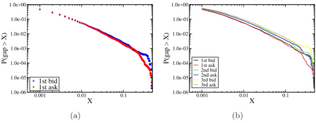
Gaps

Interestingly, the distribution of the second gaps and the third gaps in the book is very similar to that of the first gaps. The distribution of the gaps appears to show a range of scales over two decades (P(gap>X)∼X−α). We studied the distribution of the first gaps in pre-event periods and we found that the distributions on the bid and ask sides of the book differ.

Dynamics

The number of limit orders placed increases on both the bid and ask sides of the book. Regarding the dynamics of the aggregate volume of placed limit orders, we get very similar results (not shown here). The number of limit orders queued on the bid side falls to about half of the usual value and is only slowly relaxing.

An agent-based model

Details of the model

In the event of a cancellation on one side of the book, all limit orders on that side have the same probability: p=Vtotal−1 of being cancelled, where Vtotal is the total volume of limit orders on that side of the book. It is important to emphasize that in our model, traders placing limit orders refer to the mid-price, which is more realistic than referring to the previous transaction price or the best price on one side of the book. We manually generate large price changes by deleting all limit orders on one side of the book in the interval [bt−J,bt] for price declines and [at,at+J].

Figure 5.7: Scheme of the dynamics of the zero intelligence model.

Numerical results

The price axis is set very long in relation to parameter D, and can be considered infinite. As we have mentioned, with such a simple model we have to limit ourselves to the study of the bid-ask spread and the volatility, i.e. non-direct behavioral variables, in our simulated market. Similar to empirical results, the variation in volatility is much stronger than in the spread.

Analytical treatment

As we can see, the term containing the second gap appears in the expected value of the first gap. The stationary values of the spacing, first and second gaps are denoted by σ, γ(1) and γ(2), respectively. The analytical formula appears to describe spread relaxation for short times but not for long times.

Figure 5.9: The relaxation of the bid ask spread after large price changes in the model, in the limit case of P LO = 0.5, P MO = 0 and P C = 0.5

Conclusions

Settings of the experiments and information setup

To achieve equal conditions, the same dividend procedure was used for all runs of the experiment. TraderI1 knows the dividends for the end of the current period, traderI2 knows the dividends for the current and the next period,. Before starting the experiment, each trader was randomly assigned an information level from one to nine (I1, . . . ,I9), which he kept for the entire session.

Results of the experiments

At the beginning of each period, new information was delivered to the traders, depending on their information level. For the three tests, the results showed similar results to data from real markets: The distribution of returns was fat-tailed, the autocorrelation of returns decayed quickly and the autocorrelation of absolute returns decayed slowly (volatility clustering) [KH07].

Figure 6.1: Results of experiments (average of seven experiments). Return of traders relative to the market in percentage, as a function of the information

The simulations

The market mechanism and the information

When studying the performance of heterogeneously informed agents, we performed measurements with different yield processes. The results shown are the statistics of 100 simulation sessions, each run with a different random yield process. The information traders received was the present value of the stock contingent on their forecasting ability.

Trading strategies

In case of three consecutive price rises (down), they buy (sell), otherwise they place a new order in the limit order book.

Results

Final wealth as a function of information

As more agents are present in the market, the performance of the random agent approaches market return. In this case, the random trader also performs below the market level, which provides an explanation for the question raised: In the case of enough actors present on the market, the price impact of the random trader becomes negligible, so the random trader has equal probability of being beaten by the market and beating the market. To have more insight into this process, we show in Table 6.3 the relative performance of the random trader in the case of different numbers of agents (when the least informed agents are always present on the market).

Table 6.2: p–values of the Wilcoxon rank sum test for equal medians on differences in performance between the information levels

Stylized facts and efficiency

In our case, the risk-adjusted interest rate that we used to discount future dividends was set at re=0.005. It can be seen that the average of the simple net returns in the simulations is 0.0049, very close to the adjusted interest rate.

Figure 6.4: Autocorrelation functions of returns (circles and lines) and absolute returns (dots and lines) and the noise level (solid lines)

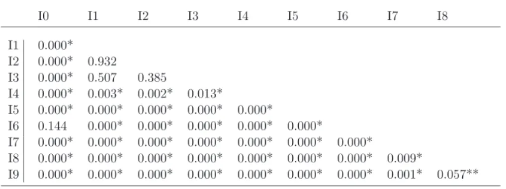
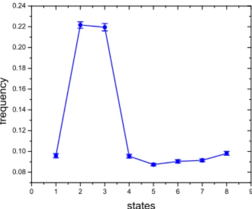
Switching strategies

Note that since agents compare their performance to the market average, the diagonal and anti-diagonal elements of the transition matrix are, by definition, zero. We find that regardless of the initial state of the system, the frequencies are approximately the same. It can be seen that most of the states appear at a low frequency regardless of the initial state.

Figure 6.6: The frequencies of states in case of three traders. The average over all possible initial states can be seen with the standard deviations as error bars

Conclusions

Much of the research has been statistical analysis of financial data, often looking for universal "stylized facts" in finance. But in the case of financial systems, unlike physical ones, we are far from having an understanding of the governing dynamics. However, due to the strong simplifying assumptions, the results were often far from the real world.

Goals

Methods

New scientific results

We have examined the distribution of the number of unoccupied price levels close to the best orders (gaps). We found that the model is able to qualitatively reproduce the slow power-law decay of the volatility and the bid-ask spread as found in empirical data. We gave an analytical form for the relaxations of the bid-ask span in the model for a limiting case and for short times in the general case [TKF08].

C´elkit˝ uz´esek

A dolgozatban igyekszem azonosítani azokat a piaci folyamatokat, amelyekben a kereskedők magatartása kulcsszerepet játszik, és azokat, amelyek ugyanazon személyek viselkedésére vonatkozó feltételezések nélkül is reprodukálhatók.

Vizsg´ alati m´ odszerek

Uj tudom´ ´ anyos eredm´enyek

Bouchaud, Herd behavior and aggregate fluctuations in financial markets, Journal of Macroeconomic Dynamics 4 (2000), no. Nijman, High-frequency analysis of lead-lag relationships among financial markets, Journal of Empirical Finance. Weiss, The continuous time random walk formalism in financial markets, Journal of Economic Behavior and Organization.