A graph is called minimally t-tough (where t is a positive real number or density) if the stickiness of the graph is exact, but removing any edge reduces the stickiness. Motivated by a theorem of Mader [24] which states that every minimally k-connected graph has a vertex of degree k (where k is a positive integer), there is a conjecture about the minimum degree of minimally sticky graphs.
Toughness
Minimally toughness
As shown by the proof, the above statement holds even if S is not a cutset. Since S is a subset inG−e, the edgee must connect two components of(G−e)−S, so e is a bridge inG−S and.
Almost minimally 1-tough graphs
Since G has at least 4 vertices, S and one of the endpoints of e form an intersection set of at most 2, soτ(G)≤1, which is a contradiction. This means that G ' K2 or G ' K3 since there are no other 1-hard graphs of at most 3 vertices with at least one edge.
Complexity
Note that, unlike t in the t-tough problem, in this problem k is part of the input. The DP completeness of the α-Critical problem is a direct consequence of the following theorem.
Thus, Dirac's theorem provides an immediate upper bound on the minimum degree of minimally 1-sticky graphs: since this theorem states that every graph at n vertices and with minimum degree contains at least n/2 a Hamiltonian cycle [14], the minimum degree of every minimally 1-tough graph is less than n/2, except for the cycle of length 4. It is not difficult to see that every minimally 1-tough graph has at least 4 vertices.
Upper bound on the minimum degree of minimally 1-tough graphs 22
Note that since the stickiness of any incomplete graph is a rational number, there exist no minimally sticky graphs with irrational stickiness. The weighted stickiness of a non-complete graph (with respect to the weight function w) is the largest twere before the graph is weighted sticky, and we declare the weighted stickiness of complete graphs (with respect to tow) as intension.
On some special cases of Theorem 4.1
On the case of minimally t -tough graphs where t is a positive
The proof of the following lemma is now omitted, but it can be found in Appendix A.1. If e does not coincide with any of the vertices of U, it connects two vertices of V.
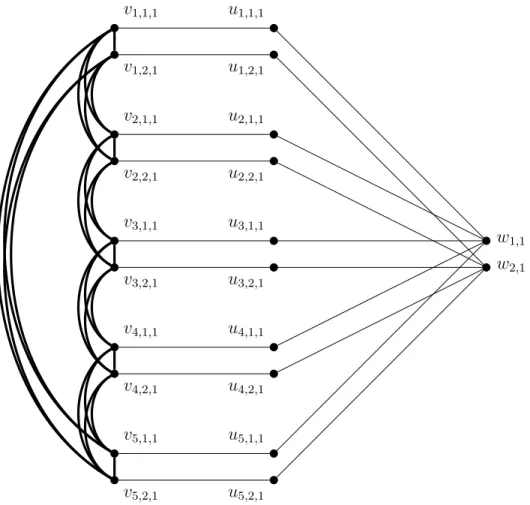
The above construction only works in case t is a positive integer for the simple reason that the sets Vi,j, Ui,j and Wj consist of t vertices. Since after gluing the vertices of G become intersection angles in the resulting graph Gt, the toughness of Gt can be at most 1/2.
In Section 4.5, the idea of the construction above is extended to the case when t≤1/2 by sticking another graph to the vertices of the original graph G. See Figure A.5.). The plan for the cases when t >1/2 is to perform this so-called glue by identifying not just one but d2th vertices of a smaller and a larger graph, where the larger graph is like a minimal-sticky graph looks and the gluing procedure aims to reduce its toughness to the desired value t.
Deleting an edge can decrease the toughness, and now we delete edges falling on W0 until the toughness remains at least t, but the deletion of any other such edge would result in a graph with toughness less than t. By repeatedly delete some edges of Ht, we eventually obtain a minimal t-hard graph, let us denote any graph obtainable in this way by Ht0 (i.e., if there exists an edge whose deletion does not reduce the toughness, then we delete that). Obviously, we could not delete the edges incident to ub, so the vertex ub still has degree 2.
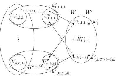
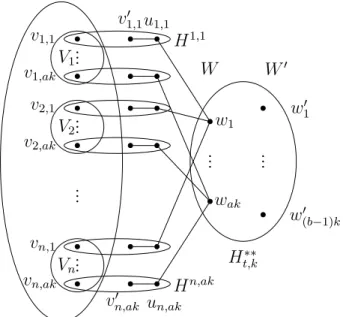
To show that G is α-critical with α(G) = k if and only if Gt,k is minimally t-solid, we first prove the following lemma. According to Proposition 2.2, for any (i, j) ∈D, removing V(Hi,j)∩S from Hi,j leaves at most di,j/t+ 1 components, but component vi,j has already been counted . By assumption (7), there is a component in Gt,k−S that contains all the remaining vertices of V∪W, and every other component is an isolated vertex of W0 (because Gt,k[W ∪W0] is a bipartite graph ) or a component of Hi,j − V(Hi,j)∩S for some i∈[n], j ∈[ak].
According to assumption (5) and Theorem 2.2 and the properties of Ht,k∗∗ (see Section 4.3.1), removing W∩S from Ht,k∗∗ leaves at most |W∩S|/t components, and one is the part of wj0. Now we return to the proof of Theorem 4.12 and show that G is α-critical with α(G) = k if and only if Gt,k is at least t-tough. According to Lemma 4.13, the graph (G−e)t,k is t-tough, but it can be obtained from Gt,k by edge deletion, which means that Gt,k is not minimally t-tough.
Minimally t -tough graphs where t ≥ 1
- The auxiliary graph H t,k ∗∗ when t ≥ 1
- The auxiliary graph H t,k 00 when t ≥ 1
- The cutsets X and Y 1 , . . . , Y T in H t 00 when t ≥ 1
- The proof of Theorem 4.1 when t ≥ 1
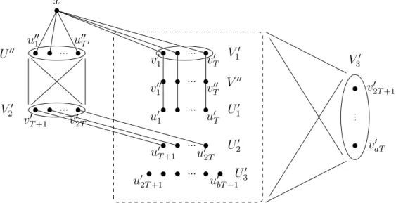
2} instead of S increases both the number of components and the weight of the removed vertex set by 1. Then if we consider the cutset S0 =S∪ {x}instead of S the number of components increases by 1 and the weight of the deleted vertex set. But by assumption (1), taking into account the cutset S0 = S∪ {vT0+l} instead of S, both the number of components and the weight of the removed topset increase by 1.
We now return to the proof of Theorem 4.18 and show that G is α-critical with α(G) =k if and only if Gt,k is minimally t-solid. By Lemma 4.19, the graph (G−e)t,k is t-solid, but it can be obtained from Gt,k by deleting edges, which means that Gt,k is not minimally t-solid. Let Almost-Min-1-Tough denote the problem of determining whether a given graph is almost minimally 1-tough.
Minimally t -tough graphs with t ≤ 1/2
The auxiliary graph H t 0 when t ≤ 1/2
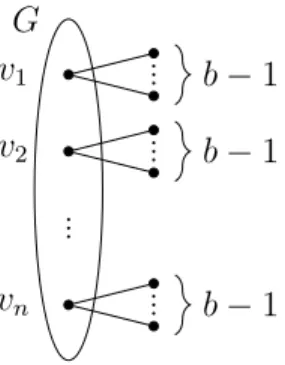
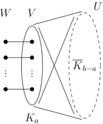
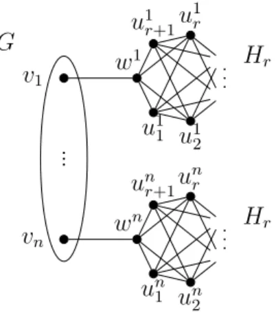
Add a clique to the vertices of V, connect each vertex of V to each vertex of U, and connect vi towi for all i∈[n]. We can assume that S∩(U ∪W) =∅ since removing any of the vertices from U ∪W does not disconnect anything in the graph. By repeatedly deleting some edges of Ht, we end up with a minimally t-tough graph; let us denote an arbitrary graph that can be obtained in this way with Ht0 (i.e. if there exists an edge whose removal does not reduce the toughness, then we remove it).
Of course, we could not delete the edges between V and W, so the vertices of W still have degree 1 in Ht0.
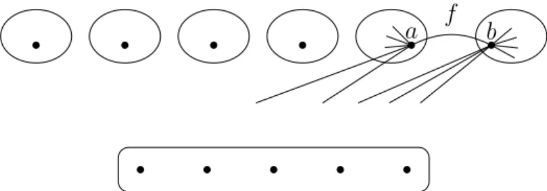
Gluing
The proof of Theorem 4.1 when t ≤ 1/2
Consider the graph Ht0 and let u∈U be an arbitrary vertex of Ht0 with degree 1, and let v be its neighbour. Now we show that G is almost at least 1-tough if and only if Gt=G⊕vHt0 is at least t-tough. So assume that e is not a bridge in Ht0 and let S =S(e)6=∅ be a vertex in Ht0 guaranteed by Theorem 2.4.
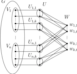
For any positive rational number t, let Exact-t-Tough-Bipartite denote the problem of determining whether a given bipartite graph has the toughest bipartite. After removing W, removing any node U∪U0 or removing only the corresponding subset Vi for any i ∈ [n] does not break anything in the graph. For every positive rational number t and positive integer l, the t-Tough problem remains coNP-complete for l-connected graphs.
The complexity of recognizing t -tough bipartite graphs
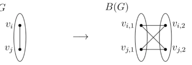
Consider the components of G0 −S0 which contain either both or none of vertices vi,1, vi,2 for anyi∈[n]. Now we reduce the DP-complete problem Exact-t/2-Tough to Exact-t-Tough-Bipartite if t < 1, and the coNP-complete problem 1/2-Tough to (Exact-)1-Tough-Bipartite . It also follows from Theorem 5.8 that recognition of t-hard bipartite graphs is coNP-complete for any positive rational number t≤1.
However, the composite bipartite graph has many degree 2 nodes due to the internal path nodes mentioned earlier, so these graphs are neither regular (except for cycles) nor 3-connected. Based on two open problems regarding the complexity of recognizing 1-tough 3-connected bipartite graphs and 1-tough 3-regular bipartite graphs [9], we also prove the following. For any fixed integer k≥2 and positive rational number t≤1, the t-Tough problem remains a coNP-complete fork-connected bipartite graph.
The complexity of recognizing t -tough k-connected bipartite graphs
The complexity of recognizing 1-tough, at least 6-regular, bipartite
We note that the reason our construction does not work in these cases is that we can decide in polynomial time whether a regular at-max 4 graph is 1/2 strong. Since removing each cut vertex disconnects the graph and thus leaves at least 2 components, the stability of the graph cannot be more than 1/2. Hence there must exist a component of G−S that has exactly one neighbor in S: since G is connected, every component has at least one neighbor in S, and if every component of G−S had at least two neighbors in S, then the number of edges going to S would be at least 2ω(G−S) > 3|S|, which would contradict the 3-regularity of G.
Then removing this vertex leaves at least three components (and note that since G is 3-regular, no more than three components can remain), so τ(G)≤1/3. In summary, it can be determined in polynomial time whether a connected 3-regular graph is 2/3 tough, and if not, then the toughness is 1/3 or 1/2. In both cases the graph contains at least one point of intersection, and if removing one of these (at least) three components remains, then the ductility of the graph is 1/3, otherwise it is 1/2.
Upper bound on the minimum degree of minimally 1-tough, bipar-
There are at most α(G) components of type (b) since the choice of a vertex of V from each such component forms an independent set G01,k[V]. Therefore, in G01,k −S there are isolated vertices of U and one more component containing the remaining vertices of W and V. In this case there are two types of components in G0t,k−S: (a) components containing only vertices of U and. b) components containing at least one vertex of V.
To obtain a component of type (a), we need to remove at least vertices of V ∪U. So there is a maximum. In G0t,k−S there are three types of components:. a) components containing at least one vertex of V, (b) isolated vertices of W,. There are thus three types of components:. a) components containing at least one vertex of V, (b) isolated vertices of W,.
Figures
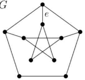
Since graph C5 is connected and α-critical with α(C5) = 2, choosing k= 2 results in a minimally 1-tough graph. Varga, A new set of basis functions for parametric curve and surface design, Proceedings of Workshop on Advances of Information Technology. Varga, On color-avoiding page complexity and link penetration, Proceedings of the 45th International Conference on Current Trends in Computer Science Theory and Practice, 2019, p.