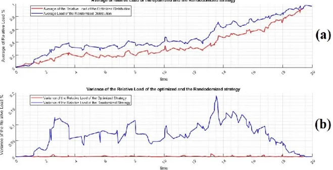
Finally, a simulation environment is designed to demonstrate the effectiveness of the proposed quantum optimization strategy. 8: (a) The average relative load of the optimized strategy (red) and the randomized one (blue). b) The variance of the relative load of the optimized strategy (red) and the randomized one (blue).
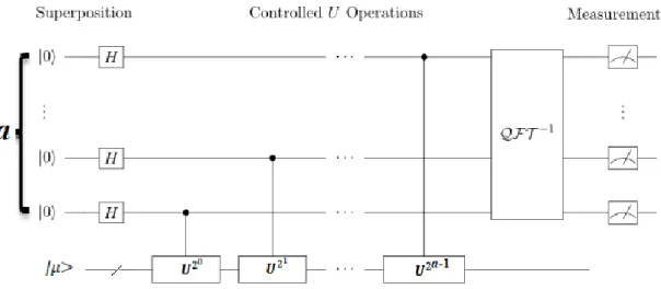
Quantum computing overview and applications
It is interesting to note that the evolution of the quantum state depends only on the start and end time. This postulate presents the concept of a quantum register that can be assembled using the tensor product of the quantum states.
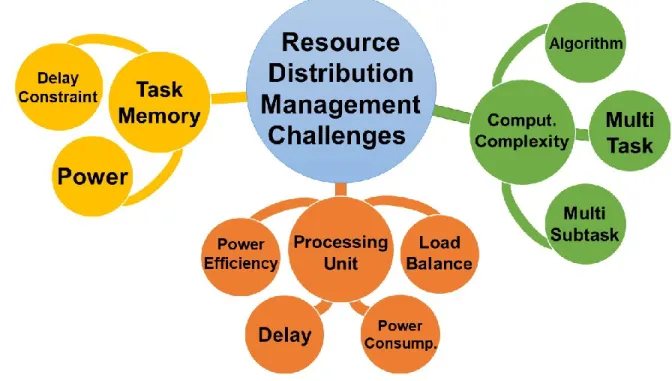
Resource distribution management and optimization methods
To show the effectiveness of the proposed quantum algorithms, the minimization of the energy consumption and the balancing of the load were considered as toy metrics. Reducing energy consumption has become a more important issue than ever due to the explosive use of the Internet and the increasing size of cloud computing.
Organization
Then, numerical results show the effectiveness of the quantum strategy in terms of load balancing and computational complexity, the results and contributions are presented in Section 3. Numerical results show that the quantum strategy is effective in terms of load balancing and computational complexity, the results and contributions are presented in Section 4.
Introduction
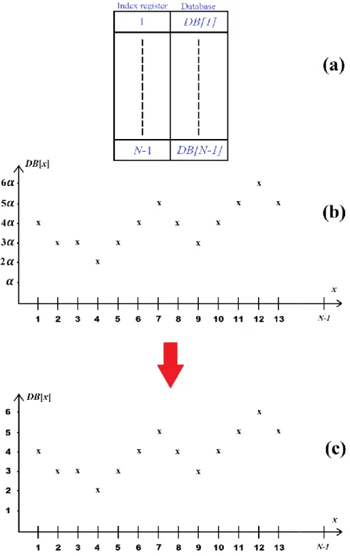
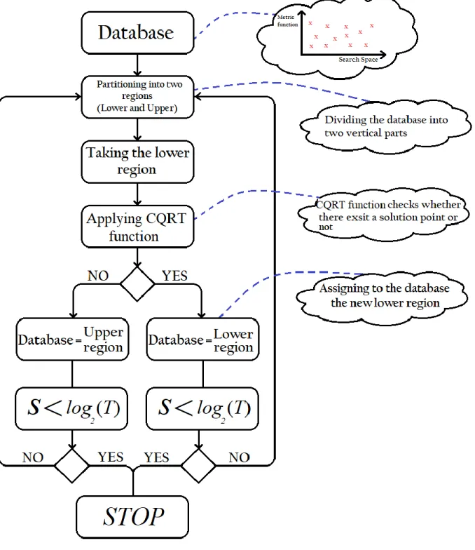
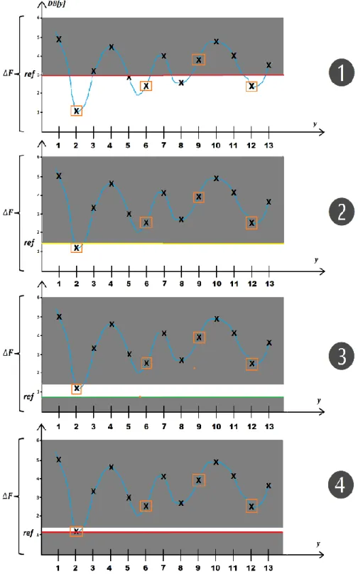
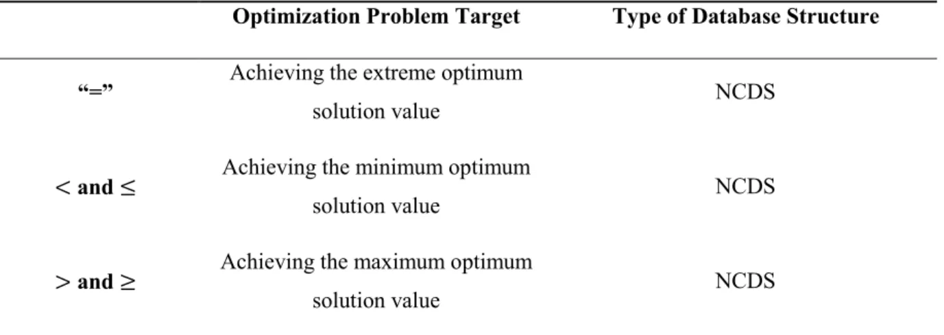
Optimization algorithms aim to find the best extreme (maximum or minimum) result of an objective function or an unselected database. An analytical comparison between the proposed QEVSA and conventional heuristic optimization algorithms is presented in Section 2.6, while Section 2.7 is a conclusion section of the chapter.
Necessary background for developing the CQOA and QOANCDS
Assume that the number of occurrences of the searched element in the database is denoted by M. We assume that the computational complexity of QEVSA is only affected by the classical security parameter.
Introducing the QOANCDS: the generalization of the quantum existence testing to
Explain why the computational complexity of the QRT is comparable to the computational complexity of QET. The computational complexity of the QRT is strongly linked to the classical and quantum uncertainty of the application.
Introducing the CQOA: the generalization of the quantum relation testing to constrained
The measurement of the phase 𝛺̃ does not affect the exact value of the constraint C. Thus, one can rewrite Eq. In other words, from Eq. 2.18), the estimation of the computational complexity of CQRT is given directly.
Comparison of the quantum optimization algorithms
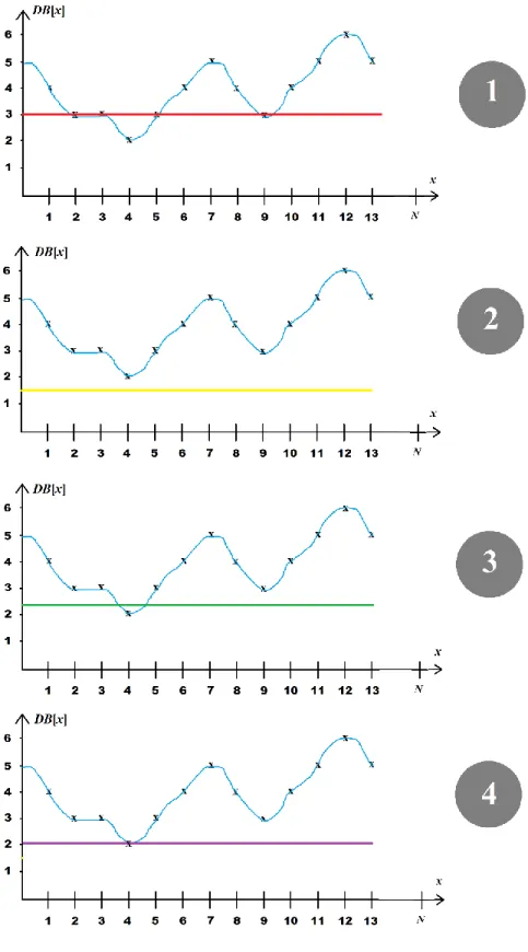
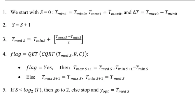
It is also important to note that the parameter T is the size of the range within the logarithm search. On the other hand, the configuration of the stochastic parameter T for QEVSA, QOANCDS and CQOA can be done using Eq.
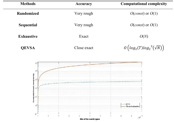
Computational complexity comparison of optimization algorithms
With regard to the randomized solution, it uses fewer steps and is thus faster than the three previous solutions, which means that the computational complexity of the randomized method is less than for the others. Moreover, it does not determine the optimal solution since the computational complexity of the sequential method is similar to that of the randomized algorithm.
Conclusion
Suppose that all classical machines that work on classical laws of classical physics disappear from our world and are replaced by quantum computers, then there is an intensive need to develop new adaptive models. Replacing the real-time decision maker with a quantum method paves the way from a resource distribution management point of view to think about how to implement a resource distribution management model with the new device, as new hardware engineering requires new modeling of the resource distribution process.
Introduction
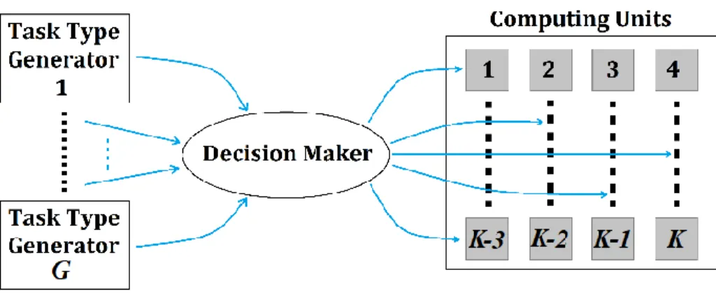
Description of the RDM system for multi-tasks
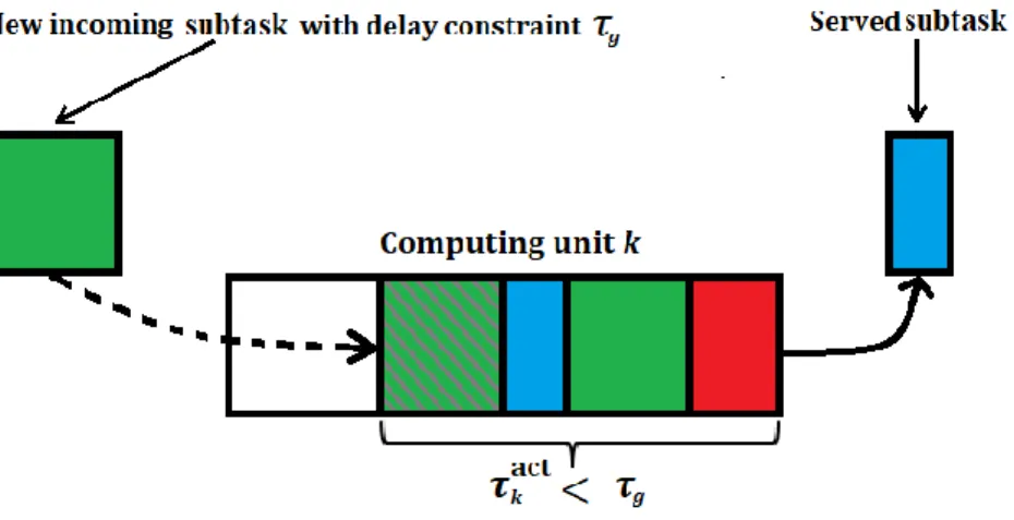
On the other hand, the processing delay of the actual load on the 𝑘𝑡ℎ computing unit can be calculated as,. It is interesting to note that the tasks are processed sequentially within the computing unit.
Implementation of the QEVSA in the RDM system for multi-tasks
Configuration of the QEVSA
3.9) The average relative load of the system when the ith computing unit receives a new input task from class 𝑠 is given as follows. The variance of the relative load of the system when the ith computing unit receives a new input task 𝑠 can be written as

Computation complexity of the QEVSA
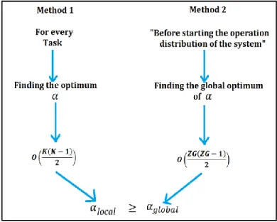
Finding the value of 𝛼𝑎𝑐𝑡𝑢𝑎𝑙 requires determining the minimum distance for any two different load distributions, expressed mathematically as 𝛼𝑎𝑐𝑡𝑎𝑢𝑙(𝑗), min. Unfortunately, there is a small drawback in the second method, if the value of 𝛼 is fixed and very small, the value of the maximum number of steps during the BSA may be larger, but it will not increase significantly, because we use the logarithmic search.
Simulation
Moreover, the simulation environment does not consider the case where the system is overloaded such that the load of the system can reach about 90%. Furthermore, it is worth noting that when the intensity distribution of tasks increases, the randomized strategy completely diverges and fluctuates dramatically, while the optimized strategy maintains and preserves the load uniformity of the system.
Conclusion
Currently, although a huge number of combinatorial methods and evolutionary algorithms have been proposed to overcome the problem of planning tasks and choose the best infrastructure for resource distribution management scheduling, it still represents a bottleneck.
Introduction
Description of RDM system for multi-tasks, multi-subtask
It is often difficult to predict the behavioral impact of a large number of resources associated with a specific treatment center.
Implementation and configuration of the QEVSA in RDM for multi-tasks, multi-
The relative load variance of the new deployment scenario is given as follows. The minimum distance between the variances of two scenarios 𝛼 is equal to zero and the values of the variables 𝑁𝑘𝑟𝑏 , 𝑣 ∈ {1,.
Computational complexity of the QEVSA
Estimation of the search space d
In the best case, the computational complexity of the constrained randomized method is O(const), and in the worst case it is O(d). The computational complexity of the constrained randomized method is O(1) or O(const), while in the worst case it is O(d) steps.
Computational complexity of calculating 𝛼
Simulation results
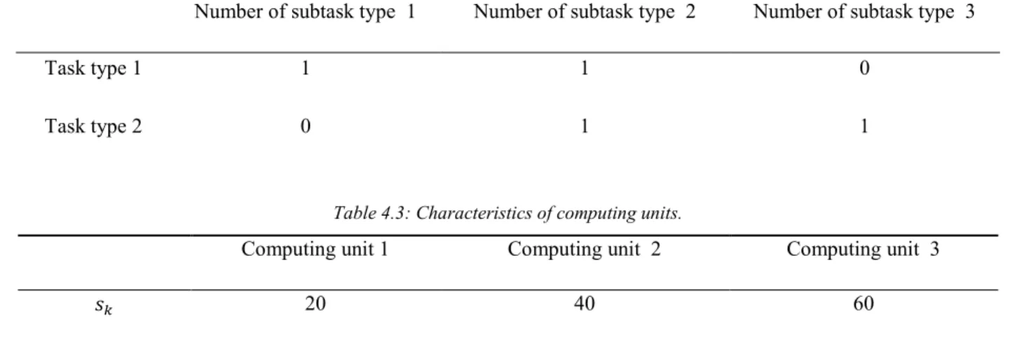
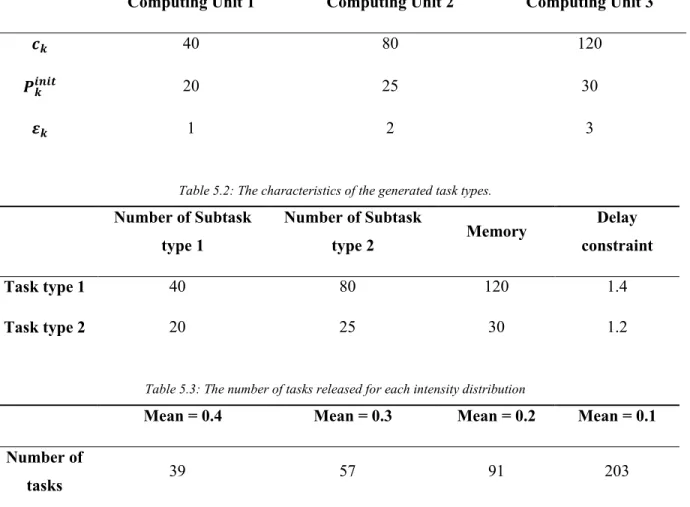
The number of subtask types in each task type is described in Table 4.2, while the characteristics of the data units are presented in Table 4.3. According to Figures 4.4 and 4.5, it is noteworthy that although the changes of the average relative load, the variance of the relative load of the optimized strategy tends to zero, while the variance of the relative load of the randomized method fluctuates and diverges from zero.
Conclusion
As is known, reducing energy consumption and improving resource utilization by taking into account the constraints arising from resource distribution management system is considered as one of the central interests of the information technology industry. To support the goals of the quality of service and the decision-making process, new computer methods must be implemented.
Introduction
Description of the RDM system for multi-tasks, multi-subtasks in case of optimizing a
The delay required to process the actual load in the 𝑘𝑡ℎ computing unit (also considering the task during the decision) denoted by 𝜏𝑘𝑎𝑐𝑡, it must always be less than or equal to the delay constraint of the incoming task type, i.e. that the actual load is interesting to note ℎ computer unit can be calculated as,.
Implementation and configuration of the CQOA
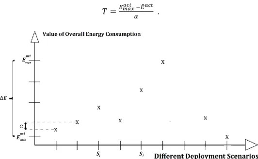
𝐸𝑚𝑎𝑥𝑖𝑛𝑐 indicates the energy consumption if the subtasks of the incoming task are deployed on those compute units with the largest 𝜀𝑘, i.e. 𝐸𝑎𝑐𝑡(𝑆𝑖) = 𝐸̆𝑎𝑐𝑡+ 𝐸 𝑖𝑛𝑐(𝑍𝑖), (5.9) where 𝑍𝑖 refers to the 𝑖𝑡ℎ collection of those compute units that receive one or more subtasks of the new incoming task.
The computational complexity of the CQOA
The size of the search space d, which refers to the total number of possible implementation scenarios, the procedure for calculating the value of d corresponds to what is shown in section 4.4.1. We confirm that the size of the search space d for the proposed constrained optimization assignment problem is similar to the previous unconstrained optimization case.
Simulation results
For example, in the first experiment, where the two task type generators have 0.4 and 0.3 respectively as the mean (the mean of exponential distribution), the energy consumption of the optimized method is less than the randomized one by approximately 43.85. As shown, the worst-case constrained randomized algorithm uses d steps, but it cannot find the optimal deployment scenarios corresponding to the minimum total energy consumption for RDMS.
Conclusion
As it is known, the length of the waiting queue and quality of service are two aspects that are linked, this is the reason why the optimization and improvement of the queuing system process is still a key focus in various application domains. For this reason, the queuing behavior appears to require more computing power than the normal deployment system.
Introduction
Description of RDM system with considering queueing scenarios
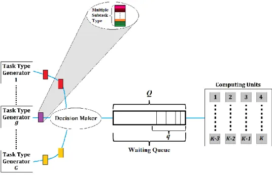
If there is free space in the compute units and the delay constraint of the incoming job is met, the subtasks derived from the incoming job are distributed to the optimal places. Assuming there is free capacity space in the 𝑘𝑡ℎ computational unit and the delay limitation applies.
Implementation, configuration, and computational complexity of the CQOA with
Shared FIFO waiting queue in the system
Let's calculate the computational complexity of the search space 𝑑 in case we consider a shared FIFO queue for all compute units and multi-task generators. Now we are able to estimate the lower and upper bounds of the search space d in the case of the multi-tasks, multi-subtasks model, where the queue type is FIFO queue.
Shared free access waiting queue in the system
To this end, the value of 𝑑 in multi-task and the multi-subtask case can be written as. In a similar way as before, to estimate the lower and the upper bounds of the search space d in the case of the multi-task, multi-subtask system, where the type of queue is free access queue, one can easily find the upper and lower bounds of Eq. 6.12) which are represented respectively as follows.
Analytical results
The proposed implemented quantum strategy relies on the CQRT derived from the quantum phase estimation, which represents the fundamental dynamo of the proposed CQOA, where it enables solving problems with exponential speedup.
Simulation Results
Case A
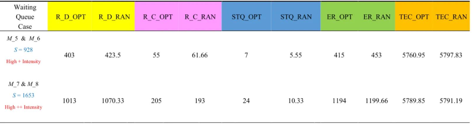
6.3, the number of rejected tasks equals zero when the intensity distribution of task types corresponding to M_1 = 0.1 and M_2 = 0.2, respectively, i.e. Moreover, it is clearly observed that the total energy consumption of the constrained randomized strategy is significantly higher than that of the constrained optimized one.
Case B
Case ANRT_OPT ANRT_RAN RfR_OPT RfR_RAN PoRT_OPT PoRT_RAN TEC_OPT TEC_RAN M_2 & M_3. ANRT_OPT: Average number of rejected jobs OPT ANRT_RAN: Average number of rejected jobs RAN RfR_OPT: Reason for rejection OPT.
Case C
6.5, when the system is overloaded, the total number of rejected tasks at the end of the simulation of the constrained randomized strategy is slightly higher than the constrained optimized one. The computational complexity of selecting the most prior task from the free access queue.
Conclusion
The fourth group of results points to the ability of the constrained quantum optimization algorithm (CQOA) to save the total constrained energy consumption of the RDM with multi-task, multi-subtasks (Chapter 5). The computational complexity of the constrained randomized is 𝑂(′𝑞), where q is the number of tasks in the queue and computational complexity of CQOA is 𝑂 (𝑙𝑜𝑔2(𝑇)𝑙𝑜(❑)𝑙𝑜)).