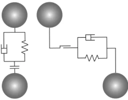
We also tested the applicability of the theory to the case of two coupled subsystems. Is it true that the movement of an individual grain of sand somehow contributes to the overall behavior of the world around us?
Granular materials
- Examples and definition
- Granular materials are athermal
- New state of matter?
- Jamming, jamming phase diagram
This structure is stable enough to support the rest of the material in the container. In the case of granular materials, jamming can only occur between random loose packing (RLP) volume fractions.
Applied methods in the study of granular materials
Particle simulation methods
Numerical modeling provides insight into the mechanisms of granular materials that are difficult or sometimes impossible to study through experiments. Therefore, one can reduce the size of the system under consideration, so that a microscopic simulation of all particles is possible.
Discrete element method simulations
An important aspect is, for example, the uniform spatial distribution of particles at the beginning of the simulation. Consequently, the interaction between particles located on opposite sides of the simulation area must be taken into account.
Dissertation objectives, outline, and contribution statement
Circle packing in two dimensions
In three dimensions for monodisperse spheres, the locally optimal configuration is the tetrahedral configuration, which does not fill space. The globally optimal configuration is the hcp or fcc structure, which has the same packing fraction (≈0.74).
Sphere packing in three dimensions
In 1890, Axel Thue proved [53] that the regular hexagonal lattice is the densest circular packing in the plane that actually has this density. Gauss proved [59] that the hcp packing is the densest packing of a lattice sphere in three-dimensional space.
Transitional regime in colloidal systems
One can obtain colloid-like behavior by introducing grain temperature, by gently shaking the system [69]. Another method is to shear the system very slowly for a long time to aid the formation of ordered layers [70].
Studied system: transition between two and three dimensions . 20
Ground state of the 2+ε-dimensional system
The analogue of a three-dimensional crystallization in hcp or fcc would be the organization of the particles in alternating bands or zigzag structures touching the back or front faces of the cell in our narrow container (see Fig. 2.5). In the second part of the chapter, I will discuss the applicability of Edwards theory to this system.
Methods
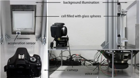
Experimental setup
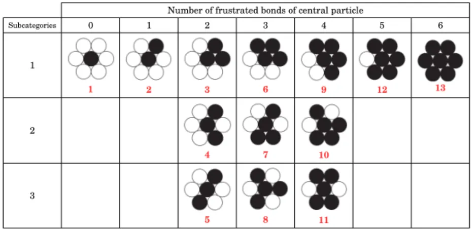
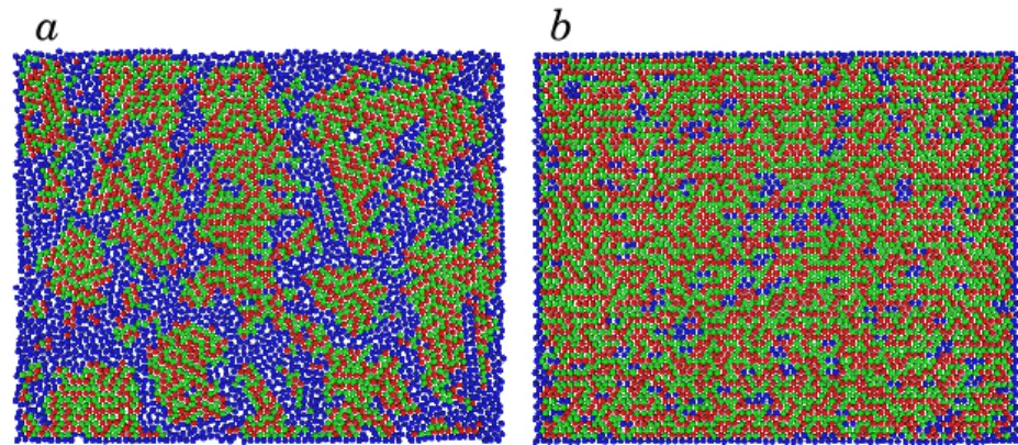
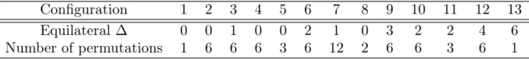
After filling by gravity from above, one finds an almost ordered arrangement, consisting of domains with a distorted triangular base lattice as seen in Fig. From the evaluated particle positions, we group the neighborhood of each sphere with 6 neighbors into the 13 different configurations shown in Fig.
Simulation setup
Blue particles are part of lattice boundaries and defects and have less than 6 neighbors, while green and red particles have 6 neighbors and they form a triangular lattice. The darker particles touch the front side of the cell while the lighter particles are located on the back side.
Results related to the time evolution
Perfectly ordered domains and lattice defects
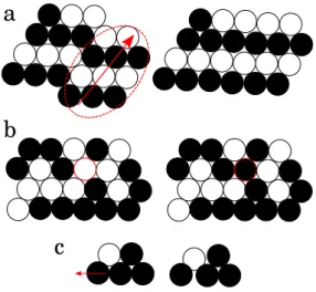
Our simulations show that defects often leave the system by forming waves (see Figure 2.10). At the same time, the volume gained by the optimized configuration is filled by particles from above.
Statistical weight of the 13 configurations
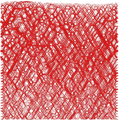
The resulting network formed by the particles may contain small defects, so the ordering is not perfect, as can be seen in the last picture of Fig. It is also noticeable especially at the bottom that most of the bars are horizontal.
Analysis of the force network
2.9 (b) shows that the outer part contains almost exclusively configurations 4 and 5, while other non-optimal ones are also visible in the central region. On average, the horizontal component of the diagonal forces equals the average horizontal force, so there is no directional bias.
Description of the system
- Analytical calculation
- Kinetic Monte Carlo simulation
- Local packing fraction model
- Combined model
- Incompatible domain structure
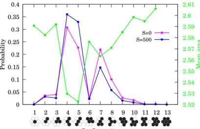
Once we have access to the minimum area that a configuration takes up, a Monte Carlo (MC) simulation of the entire system can be performed. The energy of the system is defined as the total area occupied by the configurations. Distributions of the initial state configurations of the simulations are shown in Fig.
Discussion
It is clear that the evolution of the system with ordered initial state is much slower than that of the random one. The packing fraction changes only marginally after this initial state, strengthening our previous argument about the local dynamics of the defects. This suggests that a different energy input method is needed if we want to study the frustrated dynamics of the local configurations.

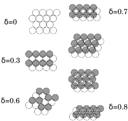
Outlook: Increasing cell thickness
Bottom: bilayer square lattice obtained in experiments with δ=0.6 and the result of the image analysis. Near-perfect two-layer structures can be seen in the case of δ=0.7 and 0.8 both in experiments and in simulations with only a few lattice defects or domain boundaries. As an example, the detection of domains with different lattice directions of a bilayer square structure in experiments is also shown in Fig.

Conclusion
The laws of “granular” thermodynamics
However, it is not clear how to distinguish between the two terms on the right side of the equation. The second law establishes the concept of entropy and states that an irreversible process in a granular system is accompanied by an increase in granular entropy: dS ≥ 0. It states that at absolute zero temperature, each thermal system is in a unique state with no entropy or with residual entropy close to zero.
Application of the theory to our system
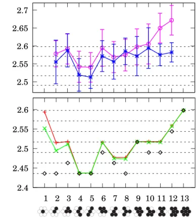
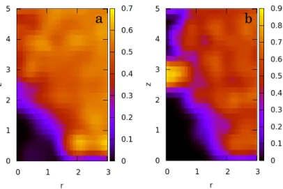
The triangular part in the case of the coupled cell experiment will be discussed later. The global volume is determined by the (x, z) positions of the particles and thus the relevant quantity is the area of the system in the x-z plane. The minimal possible Voronoi area of the central particle of the given configuration is shown by the red curve (for δ=0.3).

Methods
Experimental setup
Simulation setup
Results
- Introduction of configuration groups
- Elementary processes during shaking
- Edwards volume ensemble
- Calculations according to the canonical ensemble
- Calculations reproducing observations
- Coupling of two jammed subsystems
Process (c) has no influence on the first-order volume of δ, but contributes to the entropy of the system. In (c) and (d) the relative difference between the statistics for the fractions and the whole cell is presented. Values for the compatibility and order parameter can be found in Table 3.3 for DEM simulations.
Conclusion
Studies describing the phenomenon of clogging
An interesting aspect in the field of clogging is the description of avalanche size statistics. Avalanche size is the number or mass of particles that exit the container during an avalanche. For spheres it is the radius of the particle, and for elongated particles it is the radius of a sphere with the same volume as the elongated one.
Clogged structure in two and three dimensions
In the literature, two different approaches describing the mean size of hSi avalanches can be found. Rcis is a critical ratio of outlet radii and grains where the average size of avalanches varies. The second approach introduced by Thomas and Durian suggests an exponential relationship with the average size of avalanches.
Methods
Simulation setup
We created polydisperse samples with the variation of particle diameters by ±20%, the length of particles by ±10% and the overlap of the spheres in elongated particles between 30–50% in mean diameter units. The height of the system was much greater than the height of the resulting static granular bed, which was chosen to be approx. 25 particle diameters. Clogged states were defined by the lack of outflowing particles for a certain time to allow relaxation of the sample.
Experimental setup
Analysis methods
Results
Structure in case of spherical particles
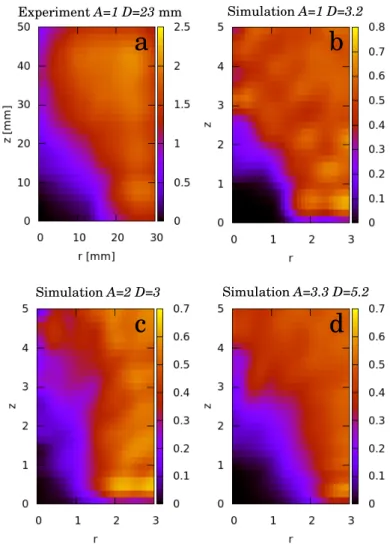
A is the aspect ratio of the particles, N is the number of occluded states considered, D/2 is the radius of the opening. The irregularity of the primary dome can be demonstrated by plotting the smooth surface generated by the triangulation method, see Fig. In this case, we applied the first approach: Points of a square grid extending in the plane of the opening were projected upwards.
Structure in case of elongated particles
As can be seen in Table 4.2, the value of (rmax−rmin)/rmin '2.5 indicates the presence of large holes in the dome. This packing can take many different sizes and can reach five times the diameter of the opening, even at moderate aspect ratios. Except for the large fluctuations found in the case of elongated particles, the detected structures support our previous finding obtained by studying the case of spherical particles, namely that the structure above the opening is made of a complex structure of two-dimensional arches.
Analysis of the force network
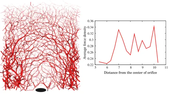
Our procedure was the following: in the case of spherical particle DEM simulations, we took parts of the force network in concentric semi-ellipsoids centered at the opening. The giant component in the first layer (red) contains the primary arc voltage across the outlet. They hold greater forces and transfer them to the bottom of the silo further from the opening.
Conclusion
Flow of granular material through an orifice
- Beverloo scaling
- Janssen effect
- Constant discharge rate of granular materials
- Effect of frictional damping and particle stiffness
Other recent studies tested the limitations, i.e., identified conditions where the flow rate is no longer constant. The introduction of an interstitial fluid clearly changes the dynamics, resulting in an increase in the flow rate near the end of the discharge process [173, 193]. We quantify the difference in laboratory experiments by measuring the flow velocity and normal force exerted on the bottom of the silo during the unloading process for both soft, low-friction grains and hard, frictional grains.
Methods
Experimental system
Also presented here are the initial silo packing fractions corresponding to fast and slow filling, ϕfast and ϕslow. We will show below that the discharge of soft hydrogel particles with low friction is very different from frictional hard grains. This motivated us to reduce the surface friction of our glass bead samples by spraying silicone oil on their surface and the silo wall.
Simulation setup
The coefficient of friction for hard surfaces with a lubricating layer depends on the normal force and the sliding velocity [207], so we performed experiments on inclined planes to measure this coefficient of friction.
Results
- Filling the silo
- Silo discharge: experiments and simulations
- Effect of friction coefficient
- Coarse-grained analysis
As discharge curves, the time evolution of the flow rate Q and the basal force Fb exerted at the bottom of the silo during discharge are considered. The effect of the interparticle friction coefficient on the flow rate is summarized in Fig. Panel (c) shows the mean value of the flow rate (for the cases where it is constant during discharge), while panel (f) shows the net gradient hdQ /dhi ·Dsilo of the flow rate (obtained by a linear fit in the range Dsilo Silicone oil is sprayed on the surface of the beads as well as on the wall of the silo. I have shown that the case of coupled subsystems can only be described by the Edwards ensemble if the stress balance at the microstate level is taken into account and the partition function of the full system is calculated. Edwards, "Geometric partition functions of cellular systems: Explicit computation of entropy in two and three dimensions", The European Physical Journal E. Martiniani, On the complexity of energy landscapes: algorithms and a direct test of the Edwards conjecture, Ph.D. A Quantitative Assessment of Flow-Induced Self-Assembly Kinetics", Journal of Colloid and Interface Science.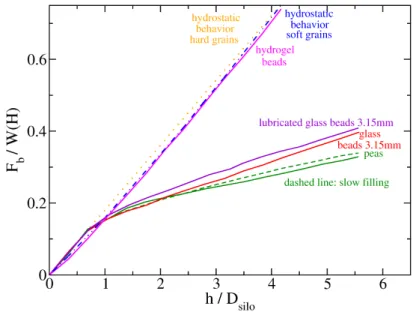
Conclusion
![Figure 1.1 Jamming phase diagrams. a: The classical diagram from Ref. [15]](https://thumb-eu.123doks.com/thumbv2/9dokorg/2496629.294066/17.892.200.747.246.502/figure-jamming-phase-diagrams-classical-diagram-ref.webp)