1
An Information-Theoretic Analysis of Resting-State versus Task fMRI
Julia Tuominen1,2, Karsten Specht1,3,4, Liucija Vaisvilaite1,3, Peter Zeidman5
1Department of Biological and Medical Psychology, University of Bergen, Bergen, Norway
2Department of Global Public Health and Primary Care, University of Bergen, Bergen, Norway
3Mohn Medical Imaging and Visualization Centre, Haukeland University Hospital, Bergen, Norway
4Department of Education, The Arctic University of Norway UiT, Tromsø, Norway
5Wellcome Centre for Human Neuroimaging, UCL Institute of Neurology, University College London, London, United Kingdom
Corresponding author:
Julia Tuominen
Department of Global Public Health and Primary Care University of Bergen
Årstadveien 17 5009 Bergen, Norway [email protected]
Keywords:
Bayesian Data Comparison, Effective connectivity, Resting-state, Task fMRI, Data quality
2 Abstract:
Resting-state fMRI is an increasingly popular alternative to task-based fMRI. However, a formal quantification of the amount of information provided by resting-state fMRI as opposed to active task conditions about neural responses is lacking. We conducted a systematic comparison of the quality of inferences derived from a resting-state- and a task fMRI paradigm by means of Bayesian Data Comparison. In this framework, data quality is formally quantified in information theoretic terms as the precision and amount of information provided by the data on the parameters of interest. Parameters of effective connectivity, estimated from the cross-spectral densities of resting-state- and task time series by means of Dynamic Causal Modelling (DCM), were subjected to the analysis. Data from 50 individuals undergoing resting-state and a Theory-of-Mind task were compared, both datasets provided by the Human Connectome Project. A threshold of very strong evidence was reached in favour of the Theory-of-Mind task (>10 bits or natural units) regarding information gain, which could be attributed to the active task condition eliciting stronger effective connectivity.
Extending these analyses to other tasks and cognitive systems will reveal whether the superior informative value of task-based fMRI observed here is case-specific or a more general trend.
3 Author Summary:
The ongoing replication crisis in neuroscience and the concurrent “paradigm shift” from task- based- to resting-state fMRI raises a question about the relative quality of the data obtained from these imaging paradigms. We compared parameters of intrinsic effective connectivity estimated from resting-state- and Theory-of-Mind datasets. The much weaker connectivity and consequent lower information gain of the resting condition was notable as the network was specified based on connectivity patterns observed under rest and consisted of regions associated with the Default-Mode-Network, which is characterized by being active during rest. These results support the assumption that the resting connectivity of the Default-Mode- Network may reflect physiological rather than neural processes, and that the neural system in question better lends itself to investigation under an active task condition.
1 1. Introduction
1
In functional magnetic resonance imaging (fMRI) research, the shift from functional
2
localization to functional- and effective connectivity as the primary object of investigation
3
has been naturally accompanied by a so-called “paradigm shift” in the design of imaging
4
protocols (Raichle, 2009). Resting-state fMRI (rs-fMRI) has become an attractive alternative
5
to task-based fMRI (t-fMRI) due to ease and efficiency of acquisition (Dubois & Adolphs,
6
2016; Leuthard et al., 2015), and because the intrinsic functional connectivity of the brain can
7
be investigated without a known timeline of experimental events (Cole et al., 2014). Yet,
8
research questions posed in the context of t-fMRI are not restricted to those pertaining to
9
functional localization. Both functional- and effective connectivity can be and are being
10
studied under different task conditions, revealing temporally coherent networks congruent
11
with those observed in rest (Calhoun et al., 2008; Cole et al., 2014; Kieliba et al., 2019; Smith
12
et al., 2009). Further, clinically relevant individual differences have been demonstrated to be
13
preserved across rest and different active tasks (Mwansisya et al., 2017; Schurz et al., 2015).
14
Followingly, the (dys)function of a given neural system can be investigated under both
15
imaging paradigms, which makes inquiries into the relative quality of the obtained data
16
highly relevant.
17
Studies that have compared the performance of t-fMRI to rs-fMRI data suggest the
18
superiority of t-fMRI in measures such as predictive accuracy and reliability (Finn et al.,
19
2017; Frässle & Stephan, 2022; Gaut et al., 2019; Greene et al., 2018; Kristo et al., 2014;
20
McCormick et al., 2022; Noble et al., 2019; Rosazza et al., 2014; Specht et al., 2003; Wang et
21
al., 2017; Weber et al., 2013, Xie et al., 2018; Yoo et al., 2018). Performance in such
22
measures is of increasing importance given the growing interest in applying fMRI in the
23
identification of disease biomarkers and in individualized treatment approaches (Brooks &
24
Vizueta, 2014; Carter et al., 2008; McDermott et al., 2018). In clinical applications the
25
2
measurement of activation strength, such as the strength of between-region coupling,
26
becomes particularly important, which introduces additional demands on data quality
27
(Specht, 2020).
28
In this study the question about data quality was formulated as to whether rs- or t-
29
fMRI data provide more information about neural responses, the relative precision with
30
which we can infer the strength of individual connection parameters, as well as the ability to
31
distinguish between different neural network architectures. These can be formally assessed
32
with an information theoretic approach in terms of reduction in entropy. The present question
33
could therefore be tackled using Bayesian Data Comparison (BDC), an analysis framework
34
introduced by Zeidman, Kazan, et al. (2019) that draws on Bayesian statistics to measure
35
movement from prior to posterior distributions afforded by the data. Neural responses,
36
defined as the rate of change in the activity of neural populations in units of s-1 (Hz), cannot
37
be directly observed using BOLD fMRI but can only be inferred under a parameterized
38
generative model. Therefore, BDC was here applied in the context of Dynamic Causal
39
Modelling (DCM) to obtain parameters of effective connectivity, which is simply the
40
contribution of one population’s neural response towards another’s. Our research question
41
can formally be stated as: how much more information do we have about the unknown
42
parameters governing neural responses after observing each kind of data.
43
The data quality indices obtained from BDC have been demonstrated to be positively
44
correlated with signal-to-noise ratio (SNR), a metric commonly used to quantify the quality
45
of fMRI data (Bennett & Miller, 2010; Welvaert & Rosseel, 2013; Zeidman, Kazan, et al.,
46
2019). However, unlike SNR that is insensitive to the feature of interest in connectivity
47
studies, the present indices measure data quality in relation to the studied connectivity
48
parameters. Thus, BDC enables an analysis of data quality beyond that indicated by SNR or
49
3
the relative amount of within- and between individual variability, which is typically
50
quantified in studies of reliability and predictive accuracy.
51
We envisage that comparing the performance of several datasets in the context of a
52
particular network model would be especially useful in clinical settings, where the focus
53
shifts from identifying the affected neural system to optimizing the imaging paradigm under
54
which to best measure its function. We hypothesized that perturbations of a neural network
55
by external stimuli, which evoke cognitive processes supported by that network, will
56
facilitate the estimation of effective connectivity parameters and lead to better performance in
57
terms of the above-mentioned quality indices. We used data from the Human Connectome
58
Project (Van Essen et al., 2013), which is particularly suitable for the present purpose due to
59
being acquired under both resting-state and different task conditions using the same
60
acquisition protocol and the same set of subjects, in addition to coming from a quality-
61
assured, open data source.
62
63
2. Materials and Methods
64
2.1. The Data.
65
We employed the minimally preprocessed data provided by the Human Connectome
66
Project (HCP). The sample consisted of 50 subjects in total, 23 males and 27 females
67
between the ages 22 and 35, selected from the predefined subset of 100 unrelated subjects of
68
the Young Adult dataset. Informed consent was obtained from the subjects both upon initial
69
screening and at the beginning of the scanning session (Van Essen et al., 2013). The present
70
study did not necessitate the use of data from siblings or twins, or biological data from HCP
71
Restricted Data, which are considered more sensitive and are available only through a
72
separate application process (Van Essen et al., 2013). Furthermore, the results will be
73
reported only at the group-level, such that any risk of identification should be minimal. The
74
4
authors of the present study have agreed to the Open Access Data Use Terms of HCP, and the
75
Norwegian Regional Committees for Medical and Health Research Ethics (REK) approved
76
the use of HCP data in the project “When Default is not Default”, of which the present study
77
is part of (REK West: 31972).
78
HCP provides data on the same subjects undergoing two rs-fMRI sessions and seven
79
t-fMRI sessions. The different tasks have been demonstrated to recruit a wide range of well-
80
characterized neural systems efficiently and reliably (Barch et al., 2013). For the current
81
analysis, we selected a social cognition task adapted from the ones developed by Castelli et
82
al. (2000) and Wheatley et al. (2007). It consists of social animation stimuli in the form of
83
video clips of geometrical objects moving either randomly or in a biologically meaningful
84
pattern, which were rated online by the participants based on whether they were perceived to
85
involve social interaction. The cognitive processes deliberately evoked by this type of task,
86
collectively known as the Theory-of-Mind (ToM), are suggested to occur spontaneously
87
during rest. Similar to other tasks engaging such “self-referential” processes, it has been
88
observed to activate parts of the Default Mode Network (DMN) (Andreasen et al., 1995;
89
Mars et al., 2012; Schilbach et al., 2008; Spreng & Grady, 2010; Spreng et al., 2009). It was
90
therefore particularly interesting to compare data from this task, hereafter referred to as the
91
ToM task, to data from a rs-fMRI session for the same group of subjects.
92
In HCP, fast sampling with TR of 720 ms and TE of 33 ms is used (Glasser et al.,
93
2013). A detailed account of the image acquisition protocol and the HCP minimal
94
preprocessing pipeline can be found in Van Essen et al. (2012) and Glasser et al. (2013). Due
95
to the specific image acquisition protocol employed in HCP there were two runs of each
96
imaging condition, scanned with reversed phase encoding directions (Van Essen et al., 2013).
97
For simplicity, in our analysis we included only data from Run 2 of the ToM task scanned in
98
the left-right direction, consisting of three clips of social interaction and two clips of random
99
5
movement. Each run started with a countdown of 8 s, and the duration of each animation clip
100
was 20 s, followed by 3 s for a behavioural response and a 15 s fixation block. One complete
101
run therefore lasted for 3 min and 27 s. Data from a resting-state (RS) session carried out on
102
the same day was utilized to avoid possible differences in the two datasets arising from
103
factors fluctuating on a daily basis. For the sake of consistency, we utilized the preprocessed
104
datasets in which ICA-based denoising has not been applied, as this option is available only
105
for rs-fMRI data. Again, data acquired with the left-right scanning direction was employed,
106
which was always the first run. The duration of the run was 14 min 33 s. In the RS condition
107
the participants were requested to lie with their eyes open and fixated on a white cross on a
108
dark background, to think of nothing particular, and not to fall asleep (Smith et al., 2013).
109
The use of concatenated images across the opposite scanning directions was assessed to
110
potentially increase overall data quality but to greatly complicate the preparatory data
111
processing without changing the relative quality of the two datasets. As our main interest was
112
in the relative and not in the absolute data quality, only the images acquired with one
113
scanning direction were included in the analysis.
114
115
2.2. Preparatory Analyses.
116
The minimally preprocessed data were smoothed with an 8mm Gaussian kernel, using
117
SPM-12 (v7771) in MATLAB 2019a. Thereafter, a standard univariate general linear model
118
(GLM) was conducted on the ToM data. In the first-level GLM analysis a design matrix was
119
specified, which included the countdown-, block-, response-, and fixation times specified
120
above. The default options of microtime resolution and -onset of 16 and 18, high-pass filter
121
128 s and canonical HRF convolution model were applied, and the 12 movement parameters
122
(translation, rotation, and their derivatives) were included as covariates in the design matrix.
123
Countdown-, fixation- and response times were included as regressors in order to obtain a
124
6
map of activation specific to viewing social stimuli. A contrast between blocks of socially
125
meaningful movement and blocks of random movement (Social > Random) was defined. In
126
the second-level group analysis a one-sample t-test was calculated for this contrast to identify
127
regions specifically and significantly responsive to social interaction. The results were
128
exported as a binary mask to be used at the subsequent stages of the analysis.
129
An independent component analysis (ICA) was conducted on the RS dataset with the
130
purpose of identifying a component that best corresponds to the activation map obtained from
131
the preceding GLM analysis, thereby thought to reflect the intrinsic connectivity of regions
132
associated with ToM processes. The RS images were also smoothed in SPM-12 with an 8
133
mm smoothing kernel before importing the files to the GIFT-toolbox v3.0b in Matlab 2019a,
134
where the ICA was performed. The number of 42 components, advocated in some sources
135
(Kiviniemi et al., 2009), was considered high enough not to result in wide, functionally
136
heterogeneous networks but neither in overly circumscribed within-region networks. The
137
default algorithm Infomax was applied. The stability of the derived components was analysed
138
with ICASSO that repeated the analysis 10 times. The spatial configurations of the
139
components were individually reconstructed and sorted according to their spatial overlap with
140
the binary mask extracted from the GLM analysis of ToM data. This allowed us to identify a
141
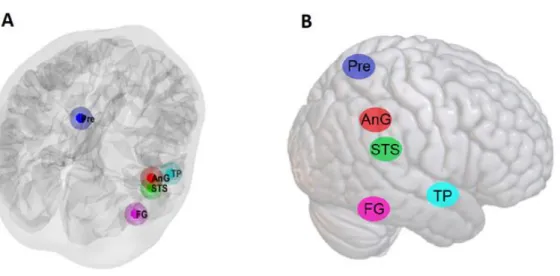
RS independent component that best overlapped with the ToM activation map. The
142
reconstructed maps of this component from each subject were imported to SPM-12, where a
143
one-sample t-test was conducted to obtain a group-level spatial map of significant clusters.
144
The coordinates of five most significant clusters were used as nodes in the following DCM
145
analysis. These five clusters are listed in Table 1.
146
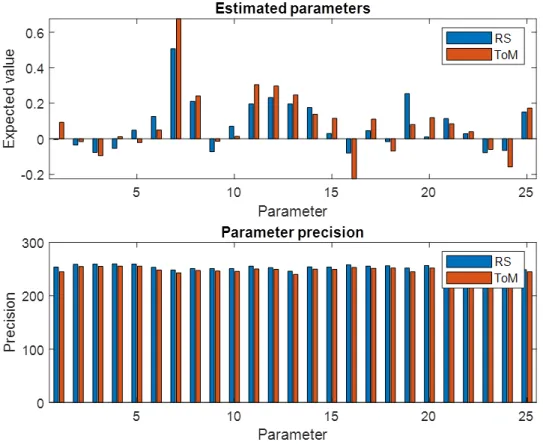
147
2.3. Main Analysis.
148
7
2.3.1. Time-series extraction. While the time courses of the ToM task were directly
149
extracted from the preparatory individual first-level GLM analysis, the RS data needed some
150
further processing. The RS time series was reduced from the original scanning length of 14
151
min 33 s to the same length as the ToM task, that is 3 min and 27 s. This ensured a more
152
formal comparison of data quality not influenced by the accumulation of signal across time,
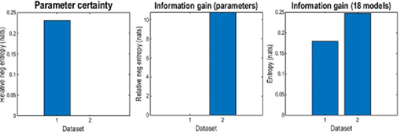
153
which is known to increase signal-to-noise ratio. As an additional analysis, we compared
154
ToM data also to the full-length RS data, as this is more consistent with the typical
155
application of rs-fMRI. First, a dummy GLM was set up to extract time series from the RS
156
data, followed by another GLM in which the twelve movement regressors and signals from
157
white matter [0, -24, -33] and cerebrospinal fluid [0, -40, -5] were used to regress out further
158
noise related to motion-, scanner- and physiological processes (Weissenbacher et al., 2009).
159
The same high-pass filter as for the ToM data analysis was applied. Time-series for the five
160
nodes were extracted by centering spherical regions with a radius of 8 mm on their
161
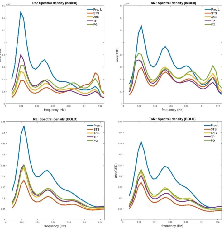
coordinates, from which the first principal eigenvariate of all voxels within the sphere,
162
centered on the peak voxel, summarized the time series of a given node. The time series were
163
mean-corrected. Motion correction and time-series extraction proceeded in a similar manner
164
for ToM data.
165
2.3.2. Dynamic Causal Modelling. The measures of data quality applied here depend
166
on both the efficiency of the selected tasks for inducing effective connectivity among the
167
regions of interest, and the efficiency of the model for inferring the presence of those effects.
168
As our focus was comparing tasks, we kept the model as consistent as possible across
169
datasets by using the same forward model with the same regions of interest and connectivity
170
architectures.
171
We employed DCM for cross-spectral densities (csd-DCM) in SPM-12 to invert a
172
neural network model consisting of the nodes identified at the preparatory stage of the
173
8
analysis (Razi et al., 2015). This was done separately for RS and ToM data, which produced
174
subject-specific estimates of intrinsic effective connectivity. DCM for CSD was used due to it
175
being applicable to both t-fMRI and rs-fMRI data (Friston et al., 2014), although this version
176
of DCM does not allow the testing of condition-specific modulations on effective
177
connectivity (i.e., no B-matrix). However, this is not relevant for the present study, where the
178
t-fMRI data only included a single experimental factor (social versus random movement).
179
Therefore, only the blocks of social stimuli were included as driving input through the
180
fusiform gyrus (C-matrix) when modelling connectivity during the ToM task. The quality
181
indices were based on the invariant connectivity (A matrix) of the respective dataset.
182
We allowed all connections between the regions to be informed by the data. In the
183
within-subject (DCM) and between-subject (Parametric Empirical Bayes, PEB) models,
184
priors on parameters were left at their default values, as supplied with the SPM12 software.
185
Priors at the within-subject subject level are detailed in Table 3 of Zeidman, Jafarian, Corbin,
186
et al. (2019) and priors at the between-subject level are detailed in Appendices 1 and 2 of
187
Zeidman, Jafarian, Seghier, et al. (2019). The most important parameters in the DCM neural
188
model for the analyses presented were those forming the region-by-region effective
189
connectivity matrix (matrix A). To briefly reprise, this was multivariate normal prior, where
190
the connection from region 𝑗 to region 𝑖 had the probability density 𝐴𝑖𝑗~𝑁(0, 1/64). This is
191
referred to as a shrinkage prior, because in the absence of evidence to the contrary, it assumes
192
no connectivity (zero Hz) among regions.
193
2.3.3. Bayesian Data Comparison. The subject-specific effective connectivity
194
parameters were subjected to the BDC analysis pipeline (spm_dcm_bdc.m, revision 7495) in
195
SPM-12. Whereas standard statistics based on likelihood ratios are used to compare the
196
evidence for different models fitted to the same data (e.g., F-tests, Bayes factors), these
197
statistics cannot be used to compare models fitted to different data. The BDC procedure
198
9
works around this by evaluating which dataset affords the greatest precision or confidence
199
about the model parameters and the models themselves. Ideally, one would follow standard
200
statistical procedure for Bayesian hypothesis testing, which is to evaluate the log evidence
201
ln 𝑃(𝑦|𝑚𝑖) for each model of interest 𝑚𝑖, and then compare them by computing the log Bayes
202
factor. For two models, the log Bayes factor is simply the difference in log evidences,
203
ln 𝑃(𝑦|𝑚1) − ln 𝑃(𝑦|𝑚2). However, this assumes that the data 𝑦 are the same for each model,
204
which precludes the use of the Bayes factor for comparing models fitted to different datasets.
205
To address this, the log evidence (and its free energy approximation used here) can be
206
decomposed into the difference between the model’s accuracy and complexity:
207
ln 𝑃(𝑦|𝑚𝑖) = 〈ln 𝑃(𝑦|𝜃, 𝑚⏟ 𝑖)〉𝑝(𝜃|𝑦,𝑚𝑖)
accuracy
− 𝐾𝐿[𝑃(𝜃|𝑦, 𝑚)||𝑃(𝜃|𝑚)]⏟
complexity 208
In words, the accuracy is the expected log likelihood (the probability of observing the
209
data under the model after estimating the parameters), which would not be meaningful to
210
compare across datasets. The complexity, also called the relative entropy, describes how far
211
the parameters have diverged from their prior expectations. This is quantified by the
212
Kullback-Leibler (KL) divergence, also called the relative entropy, which is a measure of
213
difference between two probability distributions (Joyce, 2011):
214
𝐷𝐾𝐿[𝑃(𝛽(𝑖)|𝑌(𝑖)) ∥ 𝑃(𝛽(𝑖))]
215
This quality index considers the prior and posterior expected values of the parameters
216
(𝜇0(𝑖), 𝜇(𝑖)) and the covariance matrices (Σ0(𝑖), Σ(𝑖)), which determines the effective number of
217
independent parameters that the data can support (Zeidman, Kazan, et al., 2019). This
218
measures how much information has been gained after observing the data and has natural
219
units (nats), which enable a convenient comparison between datasets. For this reason, it is
220
used in BDC as the basis for comparing how much has been learnt from each dataset. A
221
10
difference between 1.1 and 3 nats can be described as positive evidence in favour of one
222
dataset over another, a difference between 3 and 5 nats as strong evidence, and differences
223
beyond that indicate very strong evidence (akin to a Bayes Factor, Kass & Raftery, 1995).
224
The central steps of BDC are as follows. First, connection parameters are estimated
225
for each subject and are then optimized after obtaining the average connectivity of the group
226
(empirical Bayes). In more detail, for each subject 𝑠 and dataset 𝑖, a generative model of
227
fMRI data is specified:
228
vec(𝑌(𝑖,𝑠)) = 𝑓(𝜃(𝑖,𝑠)) + 𝜖(𝑖,𝑠)
229
Where 𝑌 is a matrix of fMRI timeseries data, the vec(∙) operator converts a matrix to a vector,
230
𝑓 is a model (here, an fMRI DCM), 𝜃 is a vector of connection parameters and 𝜖 are the
231
residuals. Model fitting is then performed for each subject, to obtain a posterior probability
232
distribution over the parameters, 𝑃(𝜃(𝑖,𝑠)|𝑌(𝑖,𝑠)), as well as score for the quality of the model,
233
the log evidence, which is approximated by the free energy 𝐹(𝑖,𝑠) ≈ ln 𝑃(𝑌(𝑖,𝑠)). All subjects’
234
models are then re-estimated, using the group-average connection parameters (across all
235
subjects and both datasets) as priors. This re-estimation procedure can “rescue” any subjects
236
whose parameters have fallen into different local optima.
237
Next, the optimized subject-specific connectivity parameters are summarized at the
238
group-level, separately for each dataset, using a hierarchical PEB model. This Bayesian
239
scheme provides an estimated probability distribution over the group-average connectivity
240
parameters as well as a score for the quality of the complete hierarchical model – the free
241
energy – for each dataset. These two outputs – the group-level parameters and the free energy
242
– form the basis for the comparisons that follow. More formally, for each dataset 𝑖 = 〈1,2〉
243
and subject 𝑠, we have a hierarchical model:
244
(Level 2) 𝜃(𝑖) = 𝑋𝛽(𝑖)+ 𝐸(𝑖)
245
11
(Level 1) vec(𝑌(𝑖,𝑠)) = 𝑓(𝜃(𝑖,𝑠)) + 𝜖(𝑖,𝑠)
246
Where 𝜃(𝑖) is a vector of all subjects’ connection parameters, the design matrix 𝑋
247
encodes any between-subjects effects, 𝛽 are the parameters encoding the group average
248
connectivity and the effects of any covariates on the connections, and 𝐸 is the unexplained
249
between-subjects variability. Constraints are imposed on the group-level parameters through
250
a prior probability distribution, 𝑃(𝛽(𝑖)) = 𝑁(𝜇0(𝑖), Σ0(𝑖)). Estimating the model supplies a
251
posterior probability distribution over the group-level connection parameters, informed by all
252
subjects, which is multivariate normal 𝑃(𝛽(𝑖)|𝑌(𝑖)) = 𝑁(𝜇(𝑖), Σ(𝑖)), as well as the overall free
253
energy of the hierarchical model 𝐹(𝑖) ≈ ln 𝑃(𝑌(𝑖)).
254
Three statistics are then computed in order to compare the hierarchical models fitted
255
to the different datasets, referred to as: (1) parameter certainty, (2) information gain over
256
parameters and (3) information gain over models.
257
The parameter certainty is the confidence with which the connection parameters have
258
been estimated at the group level. It is a function of the posterior covariance matrix Σ(𝑖),
259
which encodes the uncertainty or variance of each parameter on its leading diagonal, and the
260
covariance among parameters on the off-diagonal entries. The covariance determines the
261
extent to which parameters can be distinguished from each other, which is important when
262
testing hypotheses that consist of several parameters being estimated simultaneously. The
263
parameter certainty 𝑆(𝑖) is defined as the negative entropy of the covariance matrix:
264
𝑆(𝑖) = −0.5 ln|2𝜋𝑒Σ(𝑖)|
265
The dataset with highest negative entropy affords greater reduction in uncertainty,
266
measured in nats.
267
12
The information gain over parameters scores the reduction in uncertainty after seeing
268
the data relative to the uncertainty before seeing the data. It quantifies how far the parameters
269
have changed from prior beliefs 𝑃(𝛽(𝑖)) to the posterior beliefs 𝑃(𝛽(𝑖)|𝑌(𝑖)), i.e., the relative
270
entropy as explained above.
271
Finally, information gain over models indicates the ability to discriminate between
272
models and to identify the optimal one (Zeidman, Kazan, et al., 2019). In BDC, a model
273
space consisting of equally plausible but difficult to distinguish models is formed, by
274
switching on or off particular connections in the neural network. In the current case, only the
275
A-matrix from the DCM models served as input for the BDC procedure. The models are
276
assigned equal prior probabilities, forming a discrete prior probability distribution over
277
models. The posterior probability of each model is calculated, and the KL-divergence
278
between the prior and posterior probability distributions is computed (Zeidman, Kazan, et al.,
279
2019). The less uniformly the posterior probability is distributed among the models (i.e., the
280
more that some models are favoured over others), the higher KL-divergence, indicating better
281
discrimination among models and greater information gain over the model structure (See
282
Formula S1). An analytic approach for rapidly approximating the posteriors and model
283
evidence called Bayesian Model Reduction (BMR) is used to reduce computation time
284
(Friston et al., 2016).
285
In summary, the BDC procedure involves fitting models (DCMs) to each subject’s
286
fMRI data, then taking the model parameters from all subjects up to the group level and
287
fitting a GLM for each dataset under consideration. The parameters of each GLM quantifies
288
the group average connectivity, which are used to compute the statistics described above.
289
An additional step originally proposed in the BDC pipeline by Zeidman, Kazan, et al.
290
(2019) was not applied here. They used BMR to prune away any redundant parameters that
291
do not contribute to model evidence at the group-level GLM. It results in one parsimonious
292
13
model informed equally by all datasets, the parameters of which are used to re-estimate
293
individual-level connections. In this study, BDC was conducted on a fully-connected model
294
by turning off the BMR function. This was done because the network structure may differ
295
under rs- and t-fMRI and fitting the data to a model that represents a compromise between the
296
two imaging conditions might have unpredictable effects on the rest of the analysis.
297
298
3. Results
299
The comparison between the ToM activation map obtained with the GLM and the
300
forty-two RS independent components obtained with the ICA identified one component that
301
covered a substantial part of the ToM activation map. A spatial map of this component and
302
the ToM activation map are displayed in Figure 1. The activation peaks of the ToM task can
303
be found in supplementary files (Table S1). The five most significant regions identified with
304
the group-level one-sample t-test on the RS component were located in the right superior
305
temporal sulcus (rSTS), (bilateral) precuneus, right angular gyrus (rAnG), right temporal pole
306
(rTP) and right fusiform gyrus (rFG). The MNI coordinates of their cluster peaks are
307
summarized in Table 1 and approximate locations are displayed in Figure 2.
308
14
Figure 1. Activation map for the contrast Social > Random in the ToM task and the independent RS component that best overlapped with that map.
RESTING-STATE VERSUS TASK FMRI
15
309
Table 1.
Coordinates of the DCM nodes extracted from the best-matching independent component.
Label
MNI1
T-value
x y z
R angular gyrus 56 -50 20 30.94
R superior temporal sulcus 54 -46 6 25.24
R/L precuneus 4 -54 60 13.23
R temporal pole 50 -6 -18 12.44
R fusiform gyrus 44 -50 -20 7.01
1Montreal Neurological Institute brain coordinates R = Right, L = Left
16
Figure 2. A) Locations of the five nodes included in the csd-DCM on a canonical brain mesh.
B) Approximate locations of the same regions viewed from the side of the right cerebral cortex.
Figure 3. Effective connectivity during RS and ToM. The values for between-region
connections are in units of Hz whereas self-connections are unitless log-scaling values. Green and red colours represent excitatory and inhibitory connectivity, respectively. For the self- connections, positive values indicate more self-inhibition than the default value of -0.5Hz, indicated with red circles.
17
The patterns of effective connectivity among the five nodes during the ToM task and
310
during RS, directly after model inversion conducted independently on the two datasets, are
311
displayed in Figure 3. Six out of 20 between-region connections displayed reversed direction
312
of activity in terms of excitation and inhibition across the datasets. Activity within all five
313
regions had stronger self-inhibition than the default value (-0.5Hz) in both datasets.
314
The connectivity parameters, after being re-estimated with priors based on both
315
datasets, are displayed in the upper graph of Figure 4. Although the sign and relative
316
amplitude of the parameters is generally consistent between the two datasets, the majority of
317
the connections in the ToM condition moved further from the default value of zero compared
318
to RS, which indicates stronger connections in the ToM condition.
319
The parameter-specific precisions across the 25 within- and between region
320
connections, i.e., our confidence about the connection strengths after seeing the data, are
321
displayed in the lower plot of Figure 4. These precisions are defined as the inverse of the
322
posterior variance diag(Σ(𝑖))−1. It is apparent that the precisions were consistent across
323
connections and were slightly higher in the RS condition than the ToM condition. The
324
information theoretic analyses that follow quantify whether these differences across datasets
325
were non-trivial.
326
We summarised the estimated precision of the parameters across connections in terms
327
of the parameter certainty, i.e., the negative entropy, which also accounts for covariance
328
between the parameters. This was 0.23 nats in favour of the RS dataset (left panel of Figure
329
5). This difference is trivially small and not large enough to count as positive evidence
330
towards either condition. Thus, both conditions provided a similar level of confidence about
331
the estimated values of the parameters.
332
The information gain over parameters, i.e., the relative entropy from the priors to the
333
posteriors, quantifies how much has been learnt by performing the experiment in units of
334
18
nats. The difference in information gain between ToM and RS was above 10 nats and
335
qualifies as very strong evidence in favour of t-fMRI (middle panel of Figure 5). Repeating
336
the comparison using the full-length RS dataset did not noticeably change the relative
337
information gain, which remained above 10 nats in favour of ToM (Figure S1). There was
338
even a small decrease in the relative parameter certainty that was previously slightly more in
339
favour of RS.
340
Information gain depends on both the estimated strength of the connections and the
341
precision of these estimates. As the precisions did not differ meaningfully between the two
342
datasets (as quantified by the parameter certainty measure), the higher information gain
343
connected to the ToM data was primarily driven by the stronger connection strengths. This is
344
also evinced by the subject-averaged power spectrum of the estimated neural parameters
345
associated with the datasets (Figure 6), which reveal higher amplitudes across different
346
frequency bands and across most of the brain regions during the ToM task. More specifically,
347
AnG and FG display higher amplitudes in the ToM condition across all frequency bands,
348
whereas precuneus and TP display lower amplitudes only at the lowest frequency and STS at
349
the highest frequency. The power spectrum of the observed BOLD response did not differ
350
much between the datasets, except for the lowest frequency that showed higher amplitudes in
351
most of the regions in the RS dataset.
352
The right panel of Figure 5 displays the information gained by comparing several
353
equally plausible model structures. This analysis assessed whether ToM or RS data could best
354
discriminate 18 difficult to disambiguate connectivity models. The information gain over
355
model structure was 0.18 nats for RS and 0.25 nats for ToM. Both the amount of information
356
gained after model comparison and the difference between the datasets in this index were
357
negligible and do not count as evidence in favour of one or the other dataset.
358
19
Figure 4. Estimated connectivity parameters. The parameters form a multivariate normal distribution with expected values illustrated in the top plot and precisions illustrated in the bottom plot. The parameters are ordered according to outgoing connections from precuneus (bars 1-5), STS (bars 6-10), AnG (bars 11-15), TP (bars 15-19) and FG (bars 20-25). The parameters for between-region connections are rate constants with units of Hz (s-1), whereas the self-connections are unitless log-scaling parameters, which control the level of inhibition in each region. Precision is the reciprocal of variance; therefore, the units are the reciprocal of the (squared) units of the parameters.
20
Figure 5. Parameter certainty and information gain over parameters and models in units of nats. Dataset 1 stands for RS and dataset 2 for ToM. The first two indices, parameter
certainty and information gain over parameters, are negative entropies in units of nats, which are presented relative to the worst performing dataset (by subtracting the negative entropy of the best performing dataset from that of the worst performing dataset). The third index displays the amount of information gained with model comparison, separately for both datasets. Note the difference in scales – there was little difference in the parameter certainty (left) or information gain over models (right), but there was a large difference in the
information gain over parameters (middle).
21
Figure 6. The subject-averaged power spectrum of each region corresponding to the estimated neural parameters (above) and the observed BOLD response (below) during RS and ToM. The numbers from DCM.Hs were averaged and plotted against DCM.Hz. The y- axis corresponds to power and x-axis to frequency.
22 4. Discussion
359
The relative merits of using an active task versus a passive task (rest) for eliciting
360
measurable neural responses was assessed by conducting a systematic comparison of t-fMRI
361
and rs-fMRI data, in information theoretic terms. A social cognitive task evoking ToM
362
processes served as the t-fMRI condition, which was chosen on the grounds of having
363
previously demonstrated to activate brain regions attributed to the DMN (Andreasen et al.,
364
1995; Mars et al., 2012; Schilbach et al., 2008; Spreng & Grady, 2010; Spreng et al., 2009).
365
Parameters of effective connectivity derived by means of csd-DCM were subjected to the
366
analysis.
367
Activation peaks of a group-level GLM across each individual’s reconstructed RS
368
component were defined as DCM regions or nodes. The RS component was derived by
369
means of ICA and selected based on its overlap with the ToM activation map. The nodes
370
were located in rSTS, bilateral precuneus, rAnG, rTP and rFG, each of which have been
371
attributed to the DMN in earlier research (Greicius et al., 2003; Mars et al., 2012; Uddin et
372
al., 2009). None of the core hubs of DMN in the middle frontal and cingulate regions were
373
found significantly active in the current ToM task. To specifically target these regions, other
374
ToM tasks such as false belief, trait judgement, autobiographical memory, or mind-in-the-
375
eyes tasks could be considered (Andrews-Hanna et al., 2014; Schurz et al., 2014; Spreng et
376
al., 2009).
377
Results from BDC show that the ToM task condition contributed significantly more
378
information about the effective connectivity of the network model investigated here,
379
compared to RS. The difference in information gain between the two datasets can be
380
described as very strong evidence in favour of t-fMRI. Information gain depends on how far
381
the parameters have moved from their prior expectation (zero) after seeing the data, as well as
382
the confidence with which they could be estimated (their precision). In this case, the
383
23
precisions of individual parameters were similar between the two datasets, but most of the
384
connections were notably stronger in the ToM condition. This means that the higher
385
information gain in the ToM task was primarily due to the stronger effective connectivity that
386
it elicited compared to RS. Our results therefore demonstrate that the ToM task elicited
387
stronger and more readily detectable effective connectivity than RS among regions associated
388
with DMN. Connectivity strength has also been found to positively correlate with test-retest
389
reliability in effective- and functional connectivity measures (Frässle & Stephan, 2022; Noble
390
et al., 2019).
391
A useful feature of DCM is that it discriminates between neural and haemodynamic
392
components by modelling both separately to generate the observed signal, which enables the
393
inference of connectivity parameters controlling hidden or latent neural activity (Friston et
394
al., 2003; Friston et al., 2014). As the fMRI signal is an indirect measure of neural activity
395
dependent on the level of blood oxygenation (Buxton, 2013), there are concerns that some
396
patterns of connectivity are physiological rather than neural in origin (Ekstrom, 2010; Kelly
397
et al., 2012; Lurie et al., 2020). Discerning the neural signal from physiological- and
398
background noise is more challenging in rs-fMRI compared to t-fMRI due to the lack of a
399
control condition and a reference point provided by a timeline of brain activity. Also, the
400
slowly fluctuating neural activity measured in rs-fMRI may occupy the same frequency bands
401
as noise (Birn et al., 2008; Dubois & Adolphs, 2016; Liu, 2016; Reid et al., 2019), and a
402
considerable amount of rs-fMRI signal reliability and variability can be attributed to different
403
noise sources (Almgren et al., 2020; Birn et al., 2014; Sjuls & Specht, 2022; Vaisvilaite et al.,
404
2020; Wise et al., 2004; Yang et al., 2015). Consequently, the neural basis of the rs-fMRI
405
signal and its relation to cognition and behaviour are a matter of uncertainty and there is a
406
risk of confounding by physiological variables.
407
24
The results of the present analysis lend further support to this possibility, given the
408
much lower information gain connected to rs-fMRI relative to t-fMRI. This is especially
409
notable in light of two features of the present study: first, the specific network model
410
investigated in this analysis consisted of regions associated with DMN, a network thought to
411
be active during rest. Second, the nodes of the DCM were located around peak coordinates of
412
a rs-fMRI component, where only the choice of the specific component was guided by the
413
ToM activation map, hence the analysis was more biased in favour of the RS condition. The
414
power spectra in Figure 6 further emphasize the possible confounding by physiological
415
variables when investigating connectivity in rs-fMRI data. Despite the notably higher
416
amplitudes in the neural power spectrum of the t-fMRI data, differences in the observed
417
BOLD power spectrum between rs- and t-fMRI are almost indiscernible.
418
The lower information gain observed with rs-fMRI data may also partly be
419
attributable to the effect of noise correction based on signal from white matter and
420
cerebrospinal fluid. As mentioned earlier, physiological noise may occupy the same
421
frequency bands as the low frequency resting-state activity (Liu, 2016), and regressing them
422
out from the signal may also remove some of the signal of interest. A recent study
423
demonstrated that global noise regression reduced information gain but increased information
424
certainty over effective connectivity parameters (Almgren et al., 2020). It is in accordance
425
with the higher information gain connected to t-fMRI in our study, however, with the
426
difference that global signal regression is a more radical noise correction method than the one
427
applied in the present analysis. It also accords with the slightly higher certainty connected to
428
rs-fMRI, which again is explicable by the decreased within- and between variance observed
429
with such noise correction methods (Birn et al., 2014). Physiological noise and noise
430
correction are fundamental issues in fMRI data analysis, and the effect of different methods
431
25
of noise correction on both t-fMRI and rs-fMRI data can be further investigated with the
432
present information theoretic approach.
433
The final quality index, that of model discrimination ability, was low for both
434
datasets, and information gain over model structure was not significantly different across the
435
datasets. This statistic quantifies how readily similar models can be distinguished, where the
436
models differ only in whether particular connections are switched on or off (by setting
437
permissive or restrictive priors on those connections respectively). One likely explanation is
438
that switching on or off individual connections in the model made only a small difference in
439
the model evidence (free energy), due to covariance among the parameters. This may have
440
been compounded by the short length of the time series subjected to DCM analysis, relative
441
to the number of parameters in the model. Thus, finding sufficiently strong evidence for
442
switching off any individual connection would be difficult.
443
It is important to note that alternative approaches to group-level analysis of rs-fMRI
444
data may result in different peak coordinates when specifying nodes for DCM. The influence
445
of such data analysis choices on information value is an important topic to cover in future
446
studies. Further, due to our interest in quantifying information value in the context of a
447
network underlying ToM processes, we selected the rs-fMRI component that most closely
448
matched activation patterns during the ToM condition. This means that there may have
449
existed other partly overlapping rs-fMRI components with higher information value. Thus,
450
our conclusions pertain only to this particular network, and not the informative value of rs-
451
fMRI in general. More general statements about rs-fMRI will require extensive work that
452
covers different cognitive systems and networks, as well as several alternative tasks. When
453
considering the clinical utility of the imaging protocol, suitability of the task for the given
454
patient population must be considered and similar analyses repeated on patient data. Further,
455
26
the superiority of the task-fMRI data was here demonstrated with csd-DCM, and the results
456
cannot be directly generalized to other models or analysis methods.
457
458
5. Conclusion
459
The main finding of the present study is that a social cognition task (ToM) gave rise
460
to more informative inferences about the effective connectivity of regions of the DMN than
461
was enabled by rs-fMRI. The ToM task elicited stronger connections among regions
462
compared to rs-fMRI, causing an increase in the measured information gain. The brain
463
regions we examined were identified based on their activation during rs-fMRI, thus even for
464
brain regions typically associated with activation during rest, there is a compelling argument
465
for using an experimentally controlled task such as ToM to investigate them. Higher
466
information gain due to stronger effective connectivity is an advantage in situations where the
467
detectability of a network and reliability of the connectivity parameters are crucial, such as in
468
clinical contexts. The present results therefore speak for an active task condition, such as the
469
ToM task, to be preferred over rs-fMRI when investigating the (dys)function of the
470
associated neural system. The strength of DCM is that it discriminates between neural and
471
physiological sources of signal. The present results are therefore of interest also from a
472
theoretical point of view, with the much weaker connectivity observed during rest supporting
473
the assumption that the resting functional connectivity of DMN to a large part reflects
474
physiological rather than neural processes.
475
With this study we wanted to demonstrate the utility of the BDC framework for the
476
present issue and it should be considered a starting point for such analyses. The present
477
investigation may be extended to neural networks underlying other cognitive and affective
478
domains according to current theoretical and clinical research questions where the
479
development of a suitable imaging paradigm is of interest.
480
27 Data availability
481
All data were obtained from the Human Connectome Project database
482
(ConnectomeDB) and are available to investigators upon application. Analysis scripts used
483
here are available from: https://github.com/picusacademicus/RSvsToM.
484
485
Declarations of interest
486
None.
487
488
Acknowledgement
489
The study was financed by the Research Council of Norway (Project number: 276044:
490
When default is not default: Solutions to the replication crisis and beyond). Data were
491
provided by the Human Connectome Project, WU-Minn Consortium (Principal Investigators:
492
David Van Essen and Kamil Ugurbil; 1U54MH091657) funded by the 16 NIH Institutes and
493
Centers that support the NIH Blueprint for Neuroscience Research; and by the McDonnell
494
Center for Systems Neuroscience at Washington University.
495
28 References
496
Almgren, H., Van de Steen, F., Razi, A., Friston, K., & Marinazzo, D. (2020). The effect of
497
global signal regression on DCM estimates of noise and effective connectivity from
498
resting state fMRI. NeuroImage, 208, 116435.
499
https://doi.org/10.1016/j.neuroimage.2019.116435
500
Andreasen, N. C., O’Leary, D., Cizadlo, T., Arndt, S., Rezai, K., Watkins, G. L., Ponto, L. L.
501
B., & Hichwa, R. D. (1995). Remembering the past: Two facets of episodic memory
502
explored with positron emission tomography. The American Journal of Psychiatry,
503
152(11), 1576–1585. https://doi.org/10.1176/ajp.152.11.1576
504
Andrews-Hanna, J. R., Saxe, R., & Yarkoni, T. (2014). Contributions of episodic retrieval
505
and mentalizing to autobiographical thought: Evidence from functional neuroimaging,
506
resting-state connectivity, and fMRI meta-analyses. NeuroImage, 91, 324–335.
507
https://doi.org/10.1016/j.neuroimage.2014.01.032
508
Barch, D. M., Burgess, G. C., Harms, M. P., Petersen, S. E., Schlaggar, B. L., Corbetta, M.,
509
… Van Essen, D. C. (2013). Function in the human connectome: Task-fMRI and
510
individual differences in behavior. NeuroImage, 80, 169–189.
511
https://doi.org/10.1016/j.neuroimage.2013.05.033
512
Bennett, C. M., & Miller, M. B. (2010). How reliable are the results from functional magnetic
513
resonance imaging? Annals of the New York Academy of Sciences, 1191(1), 133–
514
155. https://doi.org/10.1111/j.1749-6632.2010.05446.x
515
Birn, R. M., Cornejo, M. D., Molloy, E. K., Patriat, R., Meier, T. B., Kirk, G. R., …
516
Prabhakaran, V. (2014). The Influence of Physiological Noise Correction on Test–
517
Retest Reliability of Resting-State Functional Connectivity. Brain Connectivity, 4(7),
518
511–522. https://doi.org/10.1089/brain.2014.0284
519
29
Birn, R. M., Murphy, K., & Bandettini, P. A. (2008). The effect of respiration variations on
520
independent component analysis results of resting state functional connectivity.
521
Human Brain Mapping, 29(7), 740–750. https://doi.org/10.1002/hbm.20577
522
Brooks, J. O., & Vizueta, N. (2014). Diagnostic and clinical implications of functional
523
neuroimaging in bipolar disorder. Journal of Psychiatric Research, 57, 12–25.
524
https://doi.org/10.1016/j.jpsychires.2014.05.018
525
Buckner, R. L., Andrews-Hanna, J. R., & Schacter, D. L. (2008). The Brain’s Default
526
Network: Anatomy, Function, and Relevance to Disease. Annals of the New York
527
Academy of Sciences, 1124(1), 1–38. https://doi.org/10.1196/annals.1440.011
528
Buxton, R. B. (2013). The physics of functional magnetic resonance imaging (fMRI). Reports
529
on Progress in Physics, 76(9), 096601. https://doi.org/10.1088/0034-
530
4885/76/9/096601
531
Calhoun, V. D., Kiehl, K. A., & Pearlson, G. D. (2008). Modulation of temporally coherent
532
brain networks estimated using ICA at rest and during cognitive tasks. Human Brain
533
Mapping, 29(7), 828–838. https://doi.org/10.1002/hbm.20581
534
Carter, C. S., Heckers, S., Nichols, T., Pine, D. S., & Strother, S. (2008). Optimizing the
535
Design and Analysis of Clinical Functional Magnetic Resonance Imaging Research
536
Studies. Biological Psychiatry, 64(10), 842–849.
537
https://doi.org/10.1016/j.biopsych.2008.06.014
538
Castelli, F., Happé, F., Frith, U., & Frith, C. (2000). Movement and Mind: A Functional
539
Imaging Study of Perception and Interpretation of Complex Intentional Movement
540
Patterns. NeuroImage, 12(3), 314–325. https://doi.org/10.1006/nimg.2000.0612
541
Cole, M. W., Bassett, D. S., Power, J. D., Braver, T. S., & Petersen, S. E. (2014). Intrinsic
542
and Task-Evoked Network Architectures of the Human Brain. Neuron, 83(1), 238–
543
251. https://doi.org/10.1016/j.neuron.2014.05.014
544