Complex- and hypercomplex-valued neural networks

The dynamical properties of octonic-valued neural networks are discussed in Chapter 6, which is based on 5 conference papers and 2 journal papers by the author. The content of the chapter is based on 7 conference papers and 1 journal paper of the author.

Scientific and professional results

5 papers at the International Joint Conference on Neural Networks - IJCNN (Rank A, ISI), which is the official conference of the International Neural Network Society (INNS). 1 paper at the International Conference on Artificial Neural Networks - ICANN (Rank B, ISI), which is the official conference of the European Neural Networks Association (ENNS).

Academic results

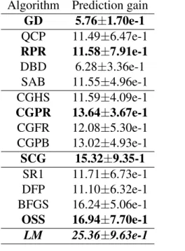
The results of the project will be incorporated into one document under development. The presentation of the improved gradient descent algorithms follows that of [180] and of the classic book [18], with the clear adaptation to the quaternion domain.

Enhanced gradient descent algorithms

• Quickprop
• Resilient backpropagation
• Delta-bar-delta
• SuperSAB

As a consequence, we had to provide separate update rules for the four components of each weight, which depend on the assumptions made about the partial derivatives of the error function with respect to each of the four components of the quaternion. Thus, SuperSAB can be seen as a combination of RPROP and delta-bar-delta algorithms.

Conjugate gradient algorithms

Instead of adding a term to the learning rate, if the partial derivatives have the same sign, as in the delta-bar-delta algorithm, we multiply it by the factor η+, as in the RPROP algorithm. Rpk+1 =−Rgk+1+βkRpk, (2.3.4) where βk ∈ Rhas different expressions, depending on the type of the conjugate gradient algorithm.

Scaled conjugate gradient method

If the error function E is quadratic, then the conjugate gradient algorithm is guaranteed to find its minimum in at most N steps. The second improvement uses a comparison parameter to evaluate how good the quadratic approximation for the error function E actually is, in the conjugate gradient algorithm.

Quasi-Newton learning methods

Now the updated expression of the inverse Hessian approximation for the symmetric rank-one (SR1) method is: As in the case of a conjugate gradient, we compute the gradient gk of the error function E by using the quaternion-valued backpropagation algorithm.

Levenberg-Marquardt learning algorithm

Unfortunately, it can be computationally intensive because it needs the explicit computation of the Hessian matrix of the error function, more precisely its inverse. This method replaces the explicit calculation of the Hessian with a calculation of the Jacobian.

Experimental results

• Linear autoregressive process with circular noise
• Discussion
• Model formulation
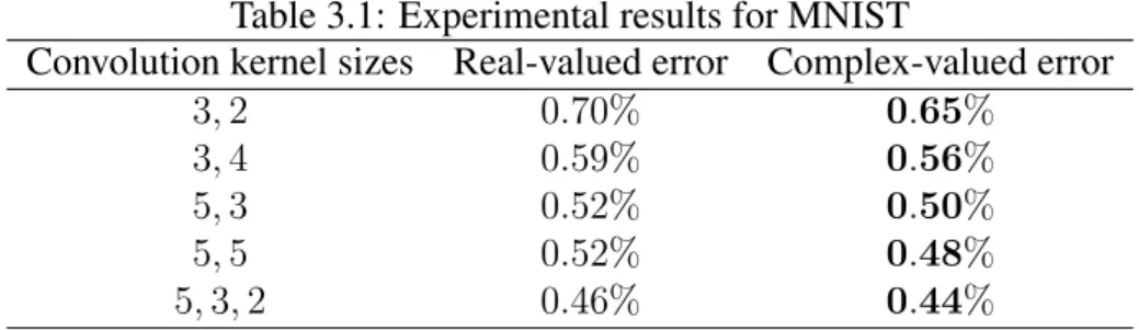
• Experimental results
• MNIST
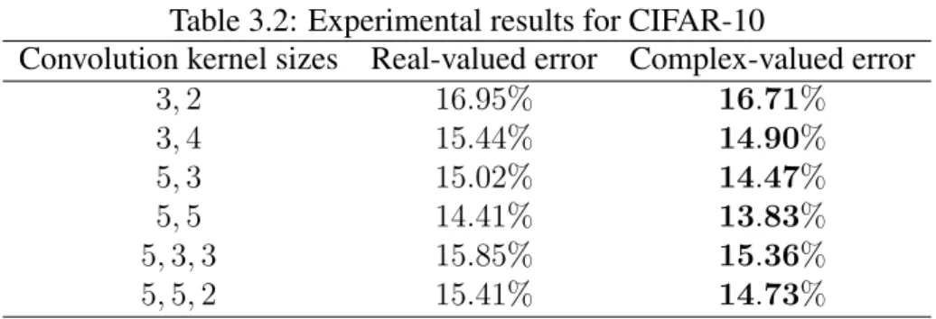
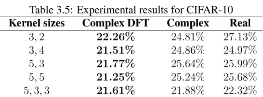
• CIFAR-10

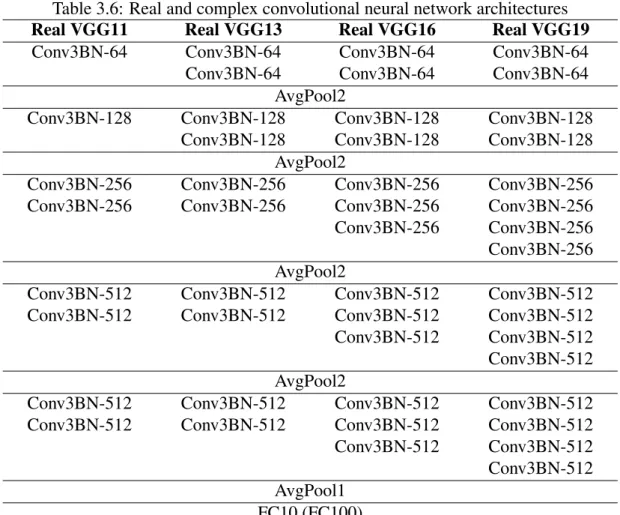
The performance of the SCG algorithm was similar to those in the previous experiments. In the context of CVCNNs, these pooling operations can only be performed separately on the real and imaginary components of the complex-valued inputs.

Fourier transform-based complex-valued convolutional neural networks

The Fourier transform

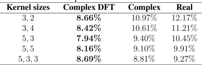
Based on these properties, the Fourier transform of an image can be shifted so that F(0,0) at the point(u0, v0) = (M/2, N/2), using the transform. This means that CVCNNs can be used to perform Fourier transform-based image classification of real value images.

Experimental results

• MNIST
• SVHN
• CIFAR-10

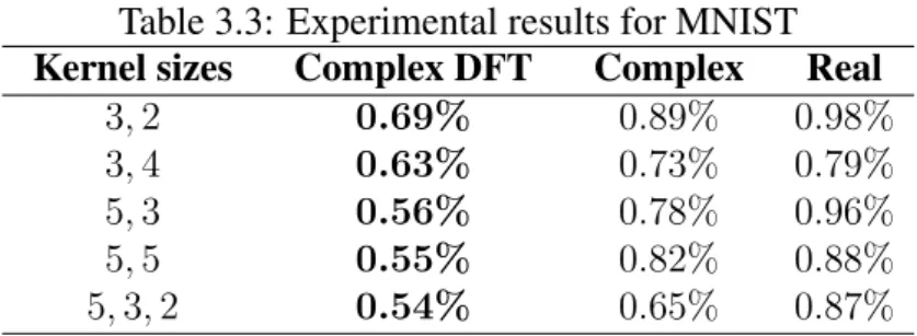
The three types of networks described above were trained on this data set, and the errors on the test set are reported in Table 3.4. But the best performance was achieved by the CVCNNs trained on the Fourier transformed images.

Deep hybrid real–complex-valued convolutional neural networks

Model formulation

For this reason, we consider a promising idea to formulate an RVCNN-CVCNN ensemble in the form of a real-complex-valued hybrid convolutional network (RCVCNN). This type of real-complex-valued hybrid ensemble is the simplest that can be formulated and constitutes the first step towards real-complex-valued hybrid networks.

Experimental results

• SVHN
• CIFAR-10
• CIFAR-100

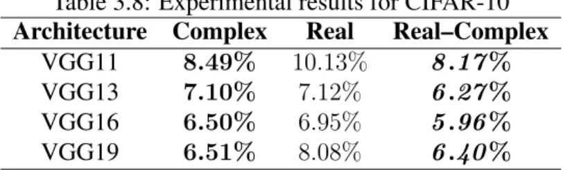
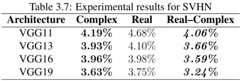
The results of training the convolutional architectures described above on this data set are given in Table 3.8 in the same format as in the previous experiment. It can be seen from the table that CVCNNs performed better than RVCNNs, but the performance increase of the hybrid ensemble was significant compared to CVCNNs.

Complex-valued stacked denoising autoencoders

Model formulation

For the complex-valued decoder, we denote by z the d-dimensional reconstruction of the representation, and add(y) the mapping that performs this reconstruction. If a good reconstruction of the input is given by the representation, then it has retained much of the information presented as input.

Experimental results

• MNIST
• FashionMNIST

Masking noise (MN), in which it is obtained by setting a part of the elements of x to 0 + 0ı= 0, randomly chosen for each example. However, the conclusion of the set of experiments is the same: complex-valued networks have better reconstruction error and better classification error than real-valued networks.

Complex-valued deep belief networks

Model formulation

The following deduction of the properties of complex-valued ring mechanisms follows that of [15] for the real-valued case. The deep belief network is thus used to initialize the parameters of the deep neural network.

Experimental results

Now that we have all the ingredients to construct and train a complex-valued RBM, we can stack multiple complex-valued RBMs to form a complex-valued deep belief network. After learning the weights of all the RBMs in the deep belief network, a logistic regression layer is added on top of the last RBM in the deep belief network, forming a complex valued deep neural network.

Complex-valued deep Boltzmann machines

Model formulation

Exact maximum likelihood learning in this model is intractable because the exact computation of data-dependent expectations is exponential in the number of hidden units, and the exact computation of model expectations is exponential in the number of visible and hidden units. The derivation of the learning procedure for complex-valued DBMs is very similar to that for complex-valued BMs and that for their real-valued counterparts given in [183, 186].

Experimental results

• MNIST
• FashionMNIST

In these applications, the stability of complex-valued neural networks plays a very important role. As a result, the study of the dynamic behavior of complex-valued recurrent neural networks has received increasing interest, especially in the last few years.

Main results

In [225] the global asymptotic stability of complex-valued BAM neural networks with constant delays was studied. Papers [38, 219] give sufficient conditions for the µ-stability of the equilibrium point of complex-valued Hopfield neural networks with unbounded time-varying delays.

Numerical examples

• Multistability analysis
• Multiperiodicity analysis

Considering that the delay kernelsKij satisfy (5.1.3) and the jump operatorsJk satisfy (5.1.4), the above system is equivalent to. The main result regarding the existence of stable states for system (5.1.1) is shown below.

Numerical examples

Quaternion-valued neural networks (QVNNs) were introduced by [4] and have applications in chaotic time series prediction [7], color image compression [89], color night vision [104], polarized signal classification [22], and 3D wind forecasting [92] , 213]. They can be applied in the signal processing domain, where certain signals can be better represented in the octonion domain.

Model formulation

We will first calculate the update rule for the weights between layerL−1 and output layer L, that is, the update rule for the weightwljk can therefore be written in octonion form in the following way: ∆wjkl (t) =−εδjlxl−1k , which is similar to the formula we obtained for the layerL.

Experimental results

• Synthetic function approximation problem I
• Synthetic function approximation problem II
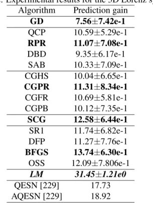
• Linear time series prediction

Octonion-valued bidirectional associative memories

Main results

In order to define the energy function for the network (6.2.1), we have to make a series of assumptions, which will be described in more detail below. The function E :ON+P → R is the energy function for the network (6.2.1) if the lead E is along the trajectories.

Asymptotic stability for OVNNs with delay

Main results

Therefore, from now on we will only study the existence, uniqueness and global asymptotic stability of the equilibrium point of the system (6.3.4). If assumption 6.1 holds, then system(6.3.4) has a unique equilibrium point that is globally asymptotically stable if there are real numbers ε1 > 0 and ε2 > 0, and a positive definite matrix P ∈R8N×8N such that the following LMI holds. 6.3.6) We will first prove that are injective.

Numerical example

Exponential stability for OVNNs with delay

Main results

Numerical example

Asymptotic stability of delayed OVNNs with leakage delay

Main results

We give a sufficient condition based on the LMI for the asymptotic stability of the origin (6.5.3). The above inequality proves the asymptotic stability of the origin of the system (6.5.3) and thus concludes the proof of the theorem.

Numerical example

Exponential stability of neutral-type OVNNs with time-varying delays

Main results

The above inequality proves the global exponential stability of the origin of the system (6.6.3), which completes the proof of the theorem. The above inequality proves the global exponential stability of the origin of the system (6.6.4), which completes the proof of the theorem.

Numerical examples

Thus, from Theorem 6.5 we can conclude that the equilibrium point of the neural network (6.6.29) with the above parameters is globally exponentially stable. It can be easily verified that Theorem 6.4 cannot be applied to Example 6.5, but Theorem 6.5 can be applied to both examples, which empirically confirms the correctness of the claims made in Remark 6.4 and Remark 6.7.

Exponential stability of OVNNs with leakage delay and mixed delays

Main results

Taking Note 6.4 into account, it can be seen that Theorem 6.6 is not equivalent to Theorem 6.7. Since Assumption 6.3 implies Assumption 6.4, but not vice versa, we can conclude that Theorem 6.7 is more general than Theorem 6.6, and for any case to which Theorem 6.6 can be applied, Theorem 6.7 can also be applied, but not otherwise.

Numerical examples

The peculiarity of the obtained results for neural networks with complex values ​​is a new contribution of the paper. First introduced by [227], complex-valued neural networks (CVNNs) have many applications, including radar imaging, antenna design, image processing, direction-of-arrival estimation and beamforming, communication signal processing, and many others [77, 78 ].

Main results

Since then, Hopfield neural networks have been applied to the synthesis of associative memories, image processing, speech processing, control, signal processing, pattern matching, etc. Due to the observations made at the beginning of this chapter, we consider an interesting idea to introduce matrix-valued Hopfield neural networks.

Matrix-valued bidirectional associative memories

Main results

Taking these assumptions into account, we can define the energy functionE :MN+Pn →R of the bidirectional associative memory (7.2.1) as:. 7.2.2) A functionE is an energy function for the network (7.2.1) as the derivative of E along the trajectories of network, denoted by dE(U(t),V(t)). In the following we will show that the function E defined in (7.2.2) is indeed an energy function for the network (7.2.1).

Asymptotic stability for MVNNs with delay

Main results

We will first transform the matrix-valued set of differential equations (7.3.1) into a real-valued set. It can be clearly seen from the above derivation that the matrix-valued recurrent neural network defined in (7.3.1) is not equivalent to an nN-dimensional real-valued recurrent neural network, because for such a network the matrices A and B are general unbounded matrices and do not have the particular form given above.

Main results

This means that the equation H(W) = 0 has a unique solution, and thus the system (7.3.4) also has a unique equilibrium point, which we will denote by Wˆ. If Assumption 7.1 holds, then the equilibrium point of the system (7.3.4) is globally asymptotically stable if there exist real numbers ε1 > 0 and ε2 > 0, and positive definite matrices P, Q, R, S∈ Mn2N such that The following LMI holds.

Numerical examples

Exponential stability for MVNNs with delay

Main results

If assumption 7.1 holds, then the origin of system (7.4.1) is globally exponentially stable if there are positive definite matrices P,Q1,Q2,Q3,S1,S2,S3,S4 and positive block diagonal matrices R1, R2. , R3, R4, all from Mn2N, and ε > 0, so that the following linear matrix inequality (LMI) is true. Taking into account this inequality (and the analog for the functions gj), and the above notations, positive block diagonal matrices exist.

Numerical example

We have thus obtained the global exponential stability for the origin of system (7.4.1). For brevity, the values ​​of the other matrices are not given.).

Exponential stability of BAM MVNNs with time-varying delays

Main results

We need to make an assumption about the activation functions to study the stability of the network defined above. Thus we obtained the exponential stability for the origin of system (7.5.5), ending the proof of the theorem.

Numerical example

Dissipativity of impulsive MVNNs with leakage delay and mixed delays

Main results

A neural network given in (7.6.4) is said to be strictly (Q,S,R)-γ-dissipative if for some γ >0 the following inequality holds under the zero initial condition:. 66]) For every positive definite matrix M ∈ Mn2N and vector function X, the following inequality holds: [a, b]→Rn. XT(s)M X(s)dsdθ where the integrals are well defined. 239]) For every positive definite matrix M ∈ Mn2N and vector function X the following inequality holds: [a, b]→Rn.

Numerical examples

YT(t)QY(t)−2YT(t)SU(t)−UT(t)(R −γIn2N)U(t) dt, which means that inequality (7.6.5) holds under zero initial condition, which implies that the neural network (7.6.4) is strictly (Q,S,R)-γ-distributive, ending the proof of the theorem.

Lie algebra-valued neural networks

Lie algebra-valued Hopfield neural networks

Lie algebra-valued bidirectional associative memories

Academic development plan

Research infrastructure