FACULTY OF MATHEMATICS AND COMPUTER SCIENCE
SCIENTIFIC REPORT
January 2016 - December 2016
MACHINE LEARNING FOR SOLVING SOFTWARE MAINTENANCE AND EVOLUTION PROBLEMS
–ˆ Inv˘ at ¸are automat˘ a ˆın probleme privind evolut ¸ia ¸ si ˆıntret ¸inerea sistemelor informatice–
Project leader: Assoc. prof. CZIBULA Istv´ an-Gergely
Project code: PN-II-RU-TE-2014-4-0082 Contract no.: 263/01.10.2015
2016
1 Introduction 2
2 Approaches for software defect detection 4
2.1 An approach usingfuzzy self-organizing maps . . . 4
2.1.1 Problem relevance. Motivation . . . 5
2.1.2 Background . . . 5
2.1.3 Methodology . . . 7
2.1.4 Computational experiments . . . 10
2.1.5 Discussion and comparison to related work . . . 13
2.1.6 Conclusions and future work . . . 15
2.2 An approach usingfuzzy decision trees . . . 15
2.2.1 Motivation . . . 16
2.2.2 Background . . . 16
2.2.3 Methodology . . . 18
2.2.4 Testing . . . 22
2.2.5 Experimental evaluation . . . 22
2.2.6 Discussion . . . 24
2.2.7 Conclusions and future work . . . 26
3 Custering based software packages restructuring 28 3.1 Motivation . . . 29
3.2 Background . . . 29
3.2.1 Clustering . . . 29
3.2.2 Software remodularization at the package level. Literature review . . . 30
3.3 Methodology . . . 31
3.3.1 Theoretical model . . . 31
3.3.2 Grouping into packages . . . 32
3.3.3 Assigning application classes to packages . . . 38
3.4 Experimental evaluation . . . 39
3.4.1 Parameters tuning . . . 39
3.4.2 Evaluation measure . . . 40
3.4.3 Experiments . . . 40
3.5 Discussion and comparison to related work . . . 53
3.5.1 Analysis of our approach . . . 53
3.5.2 Comparison to related work . . . 56
4 Hidden dependencies identification 58 4.1 Literature review . . . 58
5 Conclusions 60
1
Introduction
In this report we will present the original scientific results which were obtained for achieving the objectives proposed in the project’s work plan for the year 2016. The first scientific objective is related to thedevelopment of new classification algorithms for identifying entities with defects in software systems. The second objective is connected to the development of unsupervised learning methods for software packages restructuring. The third objective of the current project is related to conducting a literature review on hidden dependencies identification and proposing a computational model for this problem.
Chapter 2 addresses the problem of softwaredefect detection, an important problem which helps to improve the software systems’ maintainability and evolution. In order to detect defective entities within a software system, a fuzzy self-organizing feature map is proposed.
The trained map will be able to identify, using unsupervised learning, if a software module is defective or not. We experimentally evaluate our approach on three open-source case studies, also providing a comparison with similar existing approaches. The obtained results emphasize the effectiveness of using fuzzy self-organizing maps for software defect detection and confirm the potential of our proposal. Section 2.2 introduce a novel approach for predicting software defects using fuzzy decision trees. Through the fuzzy approach we aim to better cope with noise and imprecise information.A fuzzy decision tree will be trained to identify if a software module is defective or not. Two open source software systems are used for experimentally evaluating our approach. The obtained results highlight that thefuzzy decision tree approach outperforms the non-fuzzy one on almost all case studies used for evaluation. Compared to the approaches used in the literature, the fuzzy decision tree classifier is shown to be more efficient than most of the other machine learning-based classifiers.
Chapter 3 approaches the problem of software restructuring at package level which has a major importance in the field of software architecture, since refactoring increases the in- ternal software quality and is beneficial during the software maintenance and evolution. As the requirements for grouping application classes into software packages are hard to identify, clustering is useful, since it is able to uncover hidden patterns in data. In this chapter we are investigating software refactoring at the package level by using hierarchical clustering. Two approaches are proposed in order to help software developers in designing well-structured software packages. The first approach takes an existing software system and re-modularizes it at the package level using hierarchical clustering, in order to obtain better-structured pack- ages. The second method we propose considers a certain structure of packages for a software system and suggests the developer the appropriate package for a newly added application class. The experimental evaluations are performed on two open source frameworks and the algorithms have proven to perform well in comparison to existing similar approaches.
The literature review we have conducted in the direction ofhidden dependencies identifi- cation in software systems is presented in Chapter 4.
The main scientific results we have obtained during the period January 2016 - December
2
2016 are:
• An unsupervised learning based approach using fuzzy self-organizing maps (FSOM) and a supervised learning based approach using fuzzy decision trees for software defect detection.
• A hierarchical clustering based approach for software restructuring at the package level.
• 11 scientific papers (9 papers are published, 1 is accepted for publication and 1 is accepted for the second revision). From the published papers, 8 are indexed ISI (2 in SCI-E journals and 6in ISI proceedings) and 2 are BDI indexed papers.
We mention that the 2015impact factor of our ISI publications is 2.978.
Approaches for software defect detection
In this section we present our original approaches which were introduced in the direction of detecting software defects in existing software systems, usingfuzzy self-organizing maps. The original approaches were introduced by Marian, Mircea and Czibula in [72] and by Czibula, Marian and Ionescu in [30].
In order to increase the efficiency of quality assurance, defect detection tries to identify those modules of a software where errors are present. In many cases there is no time to thoroughly test each module of the software system, and in these cases defect detection methods can help by suggesting which modules should be focused on during testing.
2.1 An approach using fuzzy self-organizing maps
In order to detect faults in existing software systems, Czibula, Marian and Ionescu introduced in [30] a novel approach, based on fuzzy self-organizing feature maps. A fuzzy map will be trained, using unsupervised learning, to provide a two-dimensional representation of the faulty and non-faulty entities from a software system and it will be able to identify if a software module is or not a defective one. Five open-source case studies are used for the experimental evaluation of our approach. The obtained results are better than most of the results already reported in the literature for the considered datasets and emphasize that a fuzzy self-organizing map is more efficient than a crisp one for the case studies used for evaluation.
Software defect detection is a problem intensively investigated in the literature and an active area in the software engineering field, as shown by a systematic literature review pub- lished in 2011, which collected 208 fault prediction studies published between 2000 and 2010 [42]. Detecting software faults is a complex and difficult task, mainly for large scale soft- ware projects. In the search-based software engineering literature there are a lot of machine learning-based approaches for predicting faulty software entities, for example, [40], [76] and [66]. From a supervised learning perspective, defect prediction is a hard problem, partic- ularly because of the imbalanced nature of the training data (the number of non-defective training instances is much higher than the number ofdefective ones). Much more, it is not a trivial problem to identify a set of software metrics that would be relevant for discriminating betweenfaulty and non-faulty modules.
Even if there are a lot of methods already developed for detecting software defects, re- searchers are still focusing on improving the performance of existing classifiers. We are intro- ducing in this paper an unsupervised machine learning method based onfuzzy self-organizing mapsfor detecting faults within software systems. To the best of our knowledge, our approach is novel in the search-based software engineering literature and proved to outperform most
4
of the existing similar approaches, considering the case studies we have used for evaluation.
2.1.1 Problem relevance. Motivation
Since software systems are continuously growing in size and complexity, predicting the reli- ability of software has a fundamental role in the software development process [119]. Clark and Zubrow consider in [25] that there are three main reasons for which the analysis and prediction of software defects is essential. The first one is to help the project manager to measure the progress of a software project and to plan activities for defect detection. The second reason is to contribute to the process management, by evaluating the quality of the software product and measuring the process performance [25]. Finally, information about software faults, their location within the software and the distribution of defects may con- tribute to improving the efficiency of the testing process and the quality of the next version of a software.
Many of the machine learning-based software defect predictors existing in the literature have been built using historical data collected by mining software repositories [56]. Unfortu- nately, there are studies carried out in the defect prediction literature (like [10]) which have revealed that defect data extracted from change logs and bug reports may contain noise [56].
Other machine learning-based software defect predictors use openly available datasets, like the NASA datasets, where only the software metric values computed for the modules of the software system are available, but not the source code. Unfortunately, there can be noise in these datasets as well, as shown by [39]. Therefore, there is a need to build classifiers which can cope with the lack of information, imprecision and noise.
Fuzzytechniques are known in thesoft computing literature to be able to better deal with noisy data than the crisp methods and may lead to the development of more robust systems.
In consequence, we consider a fuzzy self-organizing map approach towards software fault detection to be a pertinent choice for both coping with uncertainty and for overcoming the drawbacks of supervised learning-based approaches (the previously mentioned problem of imbalanced data).
2.1.2 Background
In this section we aim at presenting the main characteristics of self organizing maps as well as similar approaches for software defect detection.
2.1.2.1 Fuzzy self-organizing maps
Self-organizing maps (SOMs) [98] are unsupervised learning based models from the neural networks literature that are trained using unsupervised learning to produce a two-dimensional representation of the input space (of training samples), called amap[34]. The map consists of an input layer (an input neuron for each dimension of the input data) and an array (usually two-dimensional) of neurons on the computational (output) layer. Each neuron from the input layer is connected to every output neuron and each connection is weighted.
The self-organization process consists of mapping the input instances on the neurons from output layer in order to maintain the topological relationships from the input space. The topology preservation is a main characteristic of a SOM and it means that similar input instances are mapped on neurons that are neighbors on the output map [61]. The algorithm that is usually used for training the map is the Kohonen algorithm [98]. After training, the map is able to provide clusters of similar data items [62], being appropriate for data mining tasks that require classification [62]. The SOM can be also used as effective tool for visualizing high-dimensional data.
Different approaches were developed in the literature in order to combine the theory of self-organizing maps with the theory of fuzzy sets introduced by Zadeh [117].
Tsao et. al introduced in [101] afuzzy Kohonen clustering network, combining the Fuzzy c- Means clustering (FCM) model and the Kohonen network model. This hybridization provided an optimization of the FCM, leading to an improved convergence and accuracy of the obtained results. The authors show that the proposed method can be viewed as a Kohonen type of FCM [101], the “self-organizing” character being given by the size of the updated neighborhood and the learning rate which are automatically adjusted during the learning process.
Lei and Zheng discuss in [63] the combination of ANN and fuzzy sets, and introduce a fuzzy self-organizing feature map based on Kohonen’s algorithm [63]. An output node from the map corresponds to a cluster and for each output node, a fuzzy set is defined to represent all vectors contained in the cluster corresponding to that node. Compared with the classical Kohonen algorithm, thefuzzy approach introduced in [63] replaces the distance between an input instance x and a neuron j on the map with a membership measure of x to the cluster corresponding to neuron j. The authors conclude that the resulting method, unlike the classical SOM method, is able to process inexact or fuzzy information.
Khalilia and Popescu approached in [53] the problem of clustering relational data, i.e., the problem of clustering a set of objects described by pairwise dissimilarity values. The authors proposed an algorithm, FRSOM, which is a combination of the relational SOM approach [45] (the extension of the SOM to handle relational data) and the relational fuzzy clustering algorithm presented in [46] (the extension of the fuzzy c-means algorithm to deal with relational data). The authors highlight in [53], through numerical results, that FRSOM is able to discover substructures in the data that are hard to find by the crisp relational SOM.
A very different approach was introduced by Vuorimaa in [109], a map where the nodes were replaced by fuzzy rules. The exact rules for each node are learned using the regular SOM algorithm. After the map is trained, i.e., the rules were learned, when a new instance is presented to the map, the firing strength of each rule is computed, and these strengths are used as weights to compute one final output for the map. Thus, for each input instance the map will produce one single output value.
2.1.2.2 Related work
In the following, we will briefly review several machine learning-based approaches from the defect detection literature which are somehow related to our approach (are based onunsu- pervised learning or are using the samecase studiesas in the experimental part of this paper) .
An approach that uses a combination of self-organizing maps and threshold values is presented in [5]. After the SOM is trained, threshold values are used to label the trained nodes: if any of the values from the weight vector is greater than the corresponding threshold, the node will represent the defective entities. Classification is done by finding the best matching unit for the given instance and using the label of the node.
We have introduced an approach for detecting defective entities using self-organizing maps in [75]. After an attribute selection based on the Information Gain [78] of the attributes, a map was trained to visualize the defective entities. While we had encouraging results, we have realized that in many cases defective and nondefective entities are quite similar, they are close to each other on the map. These observations led us to the use of fuzzy self-organizing maps, which can handle such situations.
There are several approaches in the literature that use different clustering algorithms to group defective and nondefective entities. One such approach is presented in [17], where K- Means algorithm is used and the centers of the clusters are found using Quad Trees. Varade and Ingle in [106] use K-Means as well, but they use Hyper-Quad Trees for the cluster center initialization. Since determining the optimal number of clusters is not a simple task, some approaches use clustering algorithms where the number of clusters is automatically determined. Such an approach is presented in [22] where the Xmeans algorithm from Weka
[41] is used for clustering. After the clusters are created software metric threshold values are used to determine which clusters represent the defective and which represent the nondefective entities. The Xmeans algorithm (together with a second clustering algorithm that is capable of automatically determining the optimal number of clusters, EM) is used by the authors in [85] as well, together with different attribute selection techniques implemented in Weka.
Yu and Mishra in [114] investigate the problem of building cross-project detection models, which are models built from data taken from one software system, but used and tested on a different software system. They use binary logistic regression on the Ar datasets, and build two models: self-assessment, when the model is tested on the dataset from which it was built, and forward-assessment, when some datasets are used for building a model and a different one is used for testing it. They conclude that self-assessment leads to better performance measures, but forward-assessment gives a more realistic measure of the real performance of the binary logistic regression model.
The problem of cross-project defect detection is approached in [81] as well. The authors consider situations when the software metrics from the datasets on which a model was built are not the same as the metrics computed for the system to be tested. They introduce an approach which tries to match the software metrics from the different sets to each other, based on correlation, distribution, and other characteristics. To compare this approach to other existing ones, they use 28 datasets (including theAr datasets) and Logistic Regression from Weka.
Multiple Linear Regression and Genetic Programming are used in [6] to evaluate the influence and performance of different resampling methods for the problem of defect detection.
TheAr datasets are used as case studies to compare five different resampling methods: hold- out, repeated random sub-sampling, 10-fold cross validation, leave-one-out cross-validation and non-parametric bootstrapping. The results of the study show that, considering the AUC performance measure, there is no significant difference between the resampling methods, but the authors claim that this can be caused by the imbalanced datasets or the high number of attributes.
A comparison of statistical and machine learning methods for defect prediction is pre- sented in [67]. They compare logistic regression with six machine learning approaches: Deci- sion Trees, Artificial Neural Networks, Support Vector Machines, Cascade Correlation Net- works, GMDH polynomial networks and Gene Expression Programming. The models were evaluated on twoAr datasets, and the best performance was obtained using Decision Trees.
2.1.3 Methodology
In this section we introduce ourfuzzy self-organizing map model for detecting faults in existing software systems.
The software entities (classes, modules, methods, functions) from a software system are represented as high-dimensional vectors (an element from this vector is the value of a software metric applied to the considered entity). As shown in [75], the software system Sof t is viewed as a set of instances (calledentities)Sof t={e1, e2, ..., en}. A set of software metrics will be used as the feature set characterizing the entities from the software system, M = {m1, m2, ..., ml}. Therefore, an entityei ∈ Sof tfrom the software system can be represented as anl-dimensional vector,ei= (ei1, ei2, . . . , eil) (eij denotes the value of the software metric mj applied to the software entityei).
For each entity from the software system, the label of the instance is known (D=defect or N=non-defect). The labels of the instances will not be used for building the fuzzy SOM model, since the learning process will be completely unsupervised. The labels will be used only for preprocessing the input data and for evaluating the performance of the resulting classification model.
Before applying the fuzzy SOM approach, the data is preprocessed. First, the data is
normalized using theMin-Max normalization method, and then a feature selection step will be used in order to identify a subset of features (software metrics) that are highly relevant for the fault detection task (details will be given in the experimental part of the paper). As a result of the feature selection step, p features (software metrics) will be selected and will be further used for building thefuzzy SOM.
2.1.3.1 The fuzzy SOM model. Our proposal
The dataset preprocessed as indicated above, will be used for the unsupervised training of the map. As for the classical SOM approach, a distance function between the input instances is needed. We are using as distance between two software entities ei and ej the Euclidean Distance between their corresponding vectors.
We are proposing, in the following, a fuzzy self-organizing map algorithm (FSOM) for building thefuzzy map. Our algorithm does not reproduce any existing algorithm from the literature, but it combines the existing viewpoints related to fuzzy SOM approaches. The underlying idea in FSOM is the classical SOM algorithm, combined with the concept of fuzziness employed infuzzy clustering [59].
The FSOM algorithm enhances the classical Kohonen algorithm for building a SOM with the idea (employed in fuzzy clustering) of using a fuzzy membership matrix. In fuzzy clustering, instead of using acrispassignment of an object to a cluster, an object can belong to multiple clusters. The degree to which an input object belongs to the clusters is indicated by the set of membership levels expressed by the columns of the membership matrix. In building thefuzzy SOM, we will use the fuzzy membership idea related to the computation of the “winning neuron”. Instead of using acrisp best-matching unit (BMU), as used in the classical SOM algorithm, the membership matrix will be used to specify the degree to which an input instance belongs to an output neuron (cluster). This means that an input instance is not mapped to a single neuron (its BMU), but to all the neurons (clusters) from the map (but with a certainmembership degree).
Intuitively, an input instance will have the larger membership degree to the neuron rep- resenting its BMU. The idea of updating the winning neuron and its neighbors is kept from the classical SOM, but if the input instance has a larger membership degree (level) to a neighboring neuron, this neuron will be “moved” closer to the input instance than the other neurons (i.e., the updating rule considers the computed membership levels). Through these updating rules, the FSOM algorithm maintains the main characteristic of the classical SOM of “moving” the winning neuron and its neighborhood towards the input instance, but it may express a better updating scheme than the crisp approach.
Let us consider, in the following, that the input layer of the map consists of p neurons (the dimensionality of the input data after the feature selection step) and the computational layer of the map consists ofcneurons disposed on a two dimensional grid, in which an output neuron i is represented as an p-dimensional vector of weights, wi = (wi1, wi2, . . . , wip) (wij represents the weight of the connection between thej-th neuron from the input layer and the i-th neuron from the computational layer).
Let us denote byuthemembership matrix, whereuik∈[0,1],∀1≤i≤c,1≤k≤n. These values are used to describe a set of fuzzy c-partitions for the n entities, and uik represents the degree to which entityek belongs to the output neuron (cluster) i.
The main steps of the FSOM algorithm are described in the following.
Step 1. Weights initialization. The weights are initialized with small random values from [0,1].
Step 2. Membership degrees computation. The values from the membership matrix are computed as in Formula (2.1) (as for thefuzzy c-means clustering algorithm [59]). m is a real number, greater than 1 and represents thefuzzifier. The role of the fuzzifier is to control
the overlapping between the clusters [59].
uik = 1
c
X
j=1
||xk−wi||
||xk−wj||
m−12
(2.1)
Step 3. Sampling. Select a random input entityetand send it to the map.
3.1 Matching. Find the “winning” neuronj∗, as the output neuron which maximizes the membership degree of the input entityet to the neuron.
3.2 Updating. After identifying the “winning neuron”, update the connection weights of the winning unit and its neighboring neurons, such that the neurons are “moved”
closer to the input instance. When updating the weights for a particular neuron, we will consider themembership degreeof the considered entity to that neuron. More precisely, for each output neuron j (∀1 ≤ j ≤ c), its weights wji (∀1 ≤ i≤ p) will be updated with a value ∆wji computed as in Formula (2.2)
∆wji=η·Tjj∗·(eti−wji)·umjt (2.2) where η is the learning rate and Tjj∗ denotes the neighborhood function usually used in the classical Kohonen’s algorithm [98] and whose radius decreases over time.
Step 4. Iteration. Repeat steps 2-3 for a given number of iterations.
If we are looking to the Step 2 of the FSOM algorithm, we observe that an input entity will have the largestmembership degree to the neuron (cluster) representing its BMU. Intuitively, the degrees to which the entity belongs to the other neurons from the map (others than its BMU) have to decrease as the distance from the entity and the neurons increases. Another characteristic of the fuzzy algorithm (compared to the crisp variant) is the fact that the weights of particular neurons from the neighborhood of the “winning neuron” (see Step 3) are updated differently depending on the degree to which the current entity belongs to the neuron. This updating method may lead to final weights which would give a better representation of the input space.
After the map was trained using the FSOM algorithm described above, in order to visual- ize the obtained map, the U-Matrix method [52] is used. The U-Matrix value of a particular node (neuron) from the map is calculated as the average distance between the node and its 4 neighbors. If one interprets these distances as heights, the U-Matrix may be interpreted as follows [52]: high places on the U-Matrix represent entities that are dissimilar with those from low places, while the data falling around the same height represent entities that are similar and can grouped together to represent a cluster.
Since the fault prediction problem is a binary classification one, our goal is to identify on the trained map two clusters corresponding to the two classes of entities: defects and non-defects.
Even if thefuzzy SOM was built using unsupervised learning, after it was created it may also be used in a supervised learning scenario for classifying a new software entity. First, the “winning neuron” corresponding to this entity is determined (as indicated at Step 3.1).
Then, the class (defect ornon-defect) to which the winning neuron belongs will indicate the result of classifying the new software entity.
For evaluating the performance of the FSOM model trained as shown above, we are com- puting the confusion matrix for the two possible classes (non-defect and defect), considering that the defective class is the positive one and the non-defective class as the negative one.
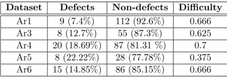
Dataset Defects Non-defects Difficulty Ar1 9 (7.4%) 112 (92.6%) 0.666 Ar3 8 (12.7%) 55 (87.3%) 0.625 Ar4 20 (18.69%) 87 (81.31 %) 0.7 Ar5 8 (22.22%) 28 (77.78%) 0.375 Ar6 15 (14.85%) 86 (85.15%) 0.666
Table 2.1: Description of the datasets used for the experimental evaluation.
For computing the values from the confusion matrix, we are using the known labels (classes) of the training entities.
Since defect prediction data are highly imbalanced (the number ofdefects is much smaller than the number ofnon-defects) the main challenge in software fault prediction is to increase the true positive rate (i.e., maximize the number of defective entities that are classified as faults), or, equivalently to decrease the false negative rate (i.e., minimize the number of de- fectiveentities that are wrongly classified asnon-faults). For the problem of defect detection, having false negatives is a more serious problem than havingfalse positives, the first situa- tion denotes an undetected fault in the system, which can cause serious problems later, while in case of the second situation some time is lost to thoroughly test a fault-free entity that was classified faulty. In the case of imbalanced data, the evaluation measure that is relevant for representing the performance of the classifiers is theArea Under the ROC Curve (AUC) measure [36] (larger AUC values indicate better classifiers).
2.1.4 Computational experiments
In this section we provide an experimental evaluation of the FSOM model (described in Section 2.2.3) on five open-source datasets which were previously used in the software defect detection literature. We mention that we have used our own implementation for FSOM, without using any third party libraries.
2.1.4.1 Datasets
The datasets used in our experiments are publicly available for download at [31] and are called Ar1, Ar3, Ar4, Ar5 and Ar6. All five datasets were obtained from a Turkish white-goods manufacturer embedded software implemented in C [75]. The software entities from these datasets are functions and methods from the considered software and are represented as 29- dimensional vectors containing the value of different McCabe and Halstead software metrics.
For each instance within the datasets, we also know the class label, denoting whether the entity isdefective ornot.
We depict in Table 2.1 the description of theAr1-Ar6 datasets used in our case studies.
For each dataset, the number ofdefectsandnon-defectsare illustrated, as well as thedifficulty of the dataset. The measure of difficulty for a dataset was introduced by Boetticher in [19]
and is computed as the percentage of entities for which the nearest neighbor (ignoring the label of the entity when computing the distances) has a different label. Since our datasets are imbalanced, when computing the difficulty of the datasets we considered only the percentage of defective entities for which the nearest neighbor is non-defective.
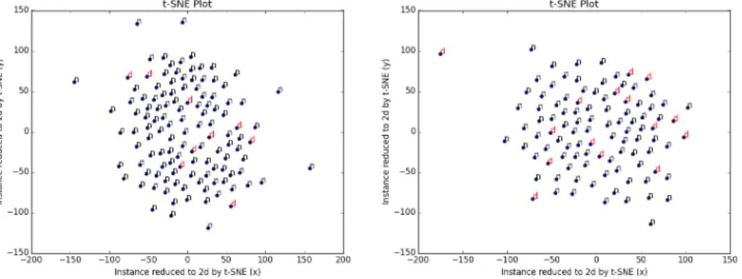
From Table 2.1 one can observe that all datasets are strongly imbalanced, with all number of defects much smaller than the number of non-defects. Moreover, it can be seen that the task of accurately classifying the defective entities is very difficult. Ar1, Ar4 and Ar6 seem to be the most difficult datasets from the defect classification point of view. The complexity of the software fault prediction task for theAr1 and Ar6 datasets is highlighted in Figures 2.1 and 2.2, which depict a two dimensional view of the data obtained using t-SNE
[104]. T-distributed Stochastic Neighbor Embedding (t-SNE) is a method for visualizing high-dimension data in a way that better reflects the initial structure of the data compared to other techniques, such as PCA. From a visualization point of view, the method has been shown to produce better results than its competitors on a significant number of datasets.
Figure 2.1: t-SNE plot for the Ar1 dataset.
Figure 2.2: t-SNE plot for the Ar6 dataset.
We can see from Figures 2.1 and 2.2 that, for both Ar1 and Ar6 datasets, the fault detection problem we are approaching in this paper is not an easy one, since it is very hard to discriminate between the defective and the non-defective entities (the non-defective entities are marked with blackn and the defective ones with redd). We have shown the t-SNE graphs only for theAr1 and Ar6 datasets, but the same situation appears for all datasets we are working with.
2.1.4.2 Results
For thefuzzy self-organizing map, we used in our experiments the torus topology, since it is shown in the literature that this topology provides better neighborhood than the conventional one [55]. The parameters used for building the map are the following: 200000training epochs and thelearning coefficient was set to 0.7. For controlling the overlapping degree in the fuzzy approach, thefuzzifier was set to 2 (shown in the literature as a good value for controlling the fuziness degree [59]).
For the feature selection step, we have used the analysis that was performed in [75] on the Ar3, Ar4 and Ar5 datasets. For determining the importance of the software metrics for the defect detection task, the information gain (IG) measure was used. From the soft- ware metrics whose IG values were higher than a given threshold, a subset of metrics that measure different characteristics of the software system were finally selected. Therefore, 9 software metrics were selected in [75] to be representative for the defect detection process:
halstead vocabulary, total operands, total operators, executable loc, halstead length, total loc, condition count,branch count,decision count [75]. The previously mentioned features (soft- ware metrics) will also be used in our FSOM approach.
We are presenting in the following the results we have obtained by applying the FSOM model (see Section 2.1.3.1) on theAr1, Ar3, Ar4,Ar5 and Ar6 datasets. After the data is preprocessed, the FSOM algorithm introduced in Section 2.1.3.1 is applied and the U-Matrix corresponding to the trained FSOM will be used to identify the class of defects and non- defects. Then, for each instance from the training dataset, we compare the class provided by our FSOM with the entity’s true class label (known from the training data). Finally, the AUC measure will be computed.
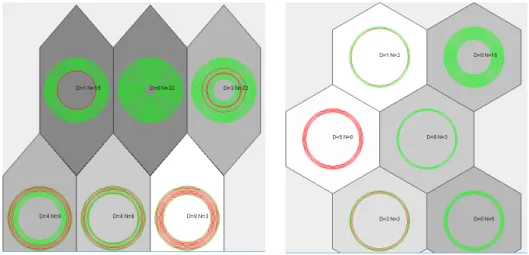
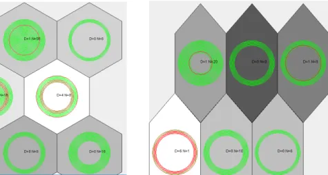
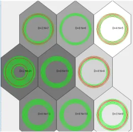
Figures 2.3, 2.4, 2.5, 2.6 and 2.7 depict the U-Matrix visualization of the best FSOMs obtained on the five datasets used in the experimental evaluation. On each neuron from the
maps we represent the training instances (software entities) which were mapped (using the FSOM algorithm) on that neuron, i.e., instances for which the neuron was their BMU. The red circles represent the defective entities and the green circles represent the non-defective entities. Each neuron is also marked with the number of defects (D) and non-defects (N) which are represented on it.
Figure 2.3: U-Matrix for the Ar1
dataset. Figure 2.4: U-Matrix for the Ar3
dataset.
Visualizing the U-Matrices from Figures 2.3, 2.4, 2.5, 2.6 and 2.7, one can identify two distinct areas: one containing lightly colored neurons, whereas the second area consists of darker neurons. The two areas represented on the maps correspond to the clusters ofdefective andnon-defective software entities. Since the percentage of software faults from the software systems is significantly smaller than the percentage of non-faulty entities (see Table 2.1), the area from the map containing a larger number of elements is considered to be thenon-defective cluster. The remaining area from the map corresponds to thedefective cluster.
Figure 2.5: U-Matrix for the Ar4 dataset.
Figure 2.6: U-Matrix for the Ar5 dataset.
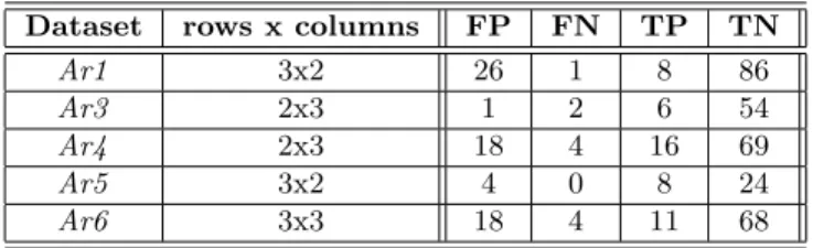
Table 3.6 illustrates, for each dataset, the configuration used for the FSOMs (number of rows and columns of the maps) as well as the values from the confusion matrix (false positives,false negatives,true positives and true negatives).
Figure 2.7: U-Matrix for theAr6 dataset.
Dataset rows x columns FP FN TP TN
Ar1 3x2 26 1 8 86
Ar3 2x3 1 2 6 54
Ar4 2x3 18 4 16 69
Ar5 3x2 4 0 8 24
Ar6 3x3 18 4 11 68
Table 2.2: Results obtained using FSOM on all experimented datasets.
2.1.5 Discussion and comparison to related work
As presented in Section 3.6 and graphically illustrated in Figures 2.3, 2.4, 2.5, 2.6 and 2.7, our FSOM approach was able to provide a good topological mapping of the entities from the software system and successfully identified two clusters corresponding to thefaulty and non-faulty entities. Even if the separation was not perfect, which is extremely difficult for the software defect detection task, for all five datasets we obtained good enoughtrue positive rates (at least 73% detection rate for the defects). For theAr5 dataset, our FSOM succeeded in obtaining a perfect defect detection rate, misclassifying only 4 non-defective entities.
The AUC measure is often considered to be the best performance measure to compare classifiers [36]. However, it is usually suitable for methods which, instead of directly returning the classification of an instance, return a score which is transformed into classification using a threshold. In such cases, different thresholds lead to different (sensitivity, 1-specificity) points on the ROC curve, and AUC measures the area under this curve. For methods where no threshold is used (for example, in our approach) the ROC curve contains one single point, which is linked to the points (0,0) and (1,1), thus providing a curve and making possible the computation of the AUC measure.
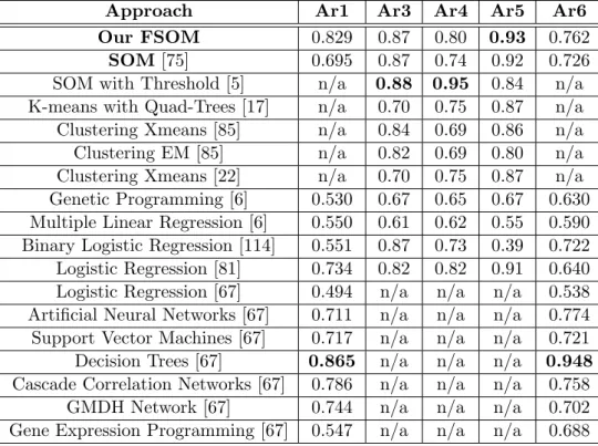
Table 2.3 presents the values of the AUC performance measure computed for the results we have obtained using our approach, but it also contains values reported in the literature for some existing similar approaches, presented in Section 2.2.2.2. If an approach does not report results on a particular dataset, we marked it with “n/a” (not available). In case of approaches that do not report the value of the AUC measure, but report other measures (for example false positive rate, false negative rate) if it was possible, we computed the values from the confusion matrix from these measures and used them to compute the value for the AUC measure, as in case of our approach. The best results obtained for the AUC measure are marked with bold in the table.
Approach Ar1 Ar3 Ar4 Ar5 Ar6 Our FSOM 0.829 0.87 0.80 0.93 0.762
SOM[75] 0.695 0.87 0.74 0.92 0.726
SOM with Threshold [5] n/a 0.88 0.95 0.84 n/a K-means with Quad-Trees [17] n/a 0.70 0.75 0.87 n/a Clustering Xmeans [85] n/a 0.84 0.69 0.86 n/a Clustering EM [85] n/a 0.82 0.69 0.80 n/a Clustering Xmeans [22] n/a 0.70 0.75 0.87 n/a Genetic Programming [6] 0.530 0.67 0.65 0.67 0.630 Multiple Linear Regression [6] 0.550 0.61 0.62 0.55 0.590 Binary Logistic Regression [114] 0.551 0.87 0.73 0.39 0.722 Logistic Regression [81] 0.734 0.82 0.82 0.91 0.640 Logistic Regression [67] 0.494 n/a n/a n/a 0.538 Artificial Neural Networks [67] 0.711 n/a n/a n/a 0.774 Support Vector Machines [67] 0.717 n/a n/a n/a 0.721 Decision Trees [67] 0.865 n/a n/a n/a 0.948 Cascade Correlation Networks [67] 0.786 n/a n/a n/a 0.758
GMDH Network [67] 0.744 n/a n/a n/a 0.702
Gene Expression Programming [67] 0.547 n/a n/a n/a 0.688 Table 2.3: Comparison of our AUC values with the related work.
We would like to mention that the results from [6] for the Multiple Linear Regression and Genetic Programming approaches are the best values reported by the authors and they were usually achieved for different resampling settings. In case of the cross-project defect prediction approach, [114], we have reported only the results of the experiments when the same dataset was used both for building the model and testing it.
From Table 2.3 we observe that our FSOM approach has better results than most of the approaches existing in the literature and considered for comparison. Out of 54 comparisons, our algorithm has a better or equal value for the AUC performance measure in 48 cases, which represents89% of the cases.
It has to be noted that thefuzzy SOM method introduced in this paper proved to have a better or equal performance, for all datasets, than thecrispapproach previously introduced in [75]. For theAr3 andAr6 datasets, the FSOM performed similarly to the classical SOM, for the other three datasets the FSOM outperformed the SOM. For theAr1 dataset, the FSOM obtained a significantly better AUC value than the classical SOM. These results highlight the effectiveness of using afuzzy approach with respect to the crisp one.
Analyzing the results from Table 2.3 we observe that our FSOM approach has the highest AUC value for theAr5 dataset, the second highest value for the Ar1 and Ar3 datasets and the third highest value for theAr6 dataset. Interestingly, the results that we have obtained are perfectly correlated with the difficulties of the considered datasets (given in Table 2.1).
More precisely, the best result was obtained for the “easiest” dataset, Ar5, while the worst results were provided for the datasets which are more “difficult”,Ar6 and Ar4. Even for the hardest datasets, the AUC values obtained by the FSOM are larger than most of the AUC values from the literature.
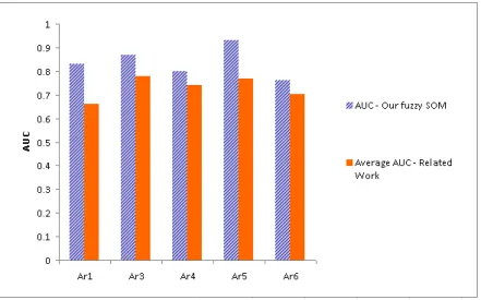
Figure 2.8 depicts, for each dataset we have considered, the AUC value obtained by our FSOM and the average AUC value reported in related work from the literature for the dataset (see Table 2.3). The first dashed bar from this figure corresponds to our FSOM. One can observe that the AUC value provided by our approach is better, for each dataset, than the average AUC value from the existing related work.
Figure 2.8: Comparison to related work.
2.1.6 Conclusions and future work
A fuzzy self-organizing feature map has been introduced in this section for detecting, in an unsupervised manner, those software entities which are likely to be defective. The experi- ments we have performed on five open-source datasets used in the software defect detection literature highlight a very good performance of the proposed approach, providing results bet- ter than most of the similar existing approaches. Moreover, thefuzzy approach introduced in this paper proved to outperform, for the considered case studies, the crisp SOM approach.
Other open-source case studies and real software systems will be further used in order to extend the experimental evaluation of the fuzzy self-organizing map model proposed in this paper. We also aim to investigate the applicability of otherfuzzy models for software defect detection (likefuzzy decision trees [116]), as well as identifying software metrics appropriate for software fault detection [90].
2.2 An approach using fuzzy decision trees
Software quality assurance is a major issue in the software engineering field and is used to ensure the software quality. In order to increase the effectiveness of quality assurance and software testing, defect prediction is used to identify defective modules in an upcoming version of a software system and is useful for assigning more effort for testing and analysing those modules [48].
Most of the machine learning based classifiers existing in the defect prediction literature are supervised. From this perspective, the problem of accurately predicting the defective modules is a hard one, because of the imbalanced nature of the training data (the number of non-defects in the the training data is much higher than the number of defects). Thus, it is hard to train a classifier to recognize the defects, when a small number of defective examples were provided during training. A major challenge in defect prediction is to increase the number of correctly identified defects and to minimize the number of misclassified defects.
Much more, it is not easy to identify the relevant software metrics which would be able to discriminate betweendefects andnon-defects.
In order to deal with the above mentioned problems, we are introducing in this section [72] a supervised machine learning method based onfuzzy decision trees for detecting defects in existing software systems. As far as we know, our approach is novel in the defect prediction literature. The experimental evaluation of the fuzzy decision tree is performed on two open
source software systems and shows that our proposal provides better results than most similar existing ones.
2.2.1 Motivation
Software defect detection represents the activity through which software modules which con- tain errors are identified. Certainly, the discovery of such defective modules plays an impor- tant role in assuring the quality of the software development process. An activity which is also connected to maintaining the software quality is the code review. Reviewing the existing code is time consuming and costly and it is frequently used in the agile software development.
Software defect detection can be helpful in the code review process to point out parts of the source code where it is likely to identify problems.
From a supervised learning perspective, the problem of identifying defective software entities is a complex and difficult one, mainly because the training data is highly imbalanced.
Obviously, a software system contains a small number of defective entities, compared to the number of non-defective ones. Thus, a supervised classifier for defect detection will be trained with a set of defective examples which is much smaller than the set of non-defective ones.
This way, the classifier would be susceptible to learn to assign the majority class, namely the non-defective class. That is why, the field of software defect prediction is a very active research area, being a continuous interest in developing performant classifiers which are able to handle the imbalanced nature of the software defect data.
Several studies that have been performed in the defect prediction literature [10] have shown that defect data extracted from change logs and bug reports may be noisy and imprecise [56]. Our previous research in the defect prediction field (like [75]) reinforced the idea that it is very hard to find a crisp separation between the defective and non-defective entities, in most situations defective entities seem to be very similar to non-defective ones. The self-organizing map used in [75] revealed that the defect data contains some uncertain areas (overlapping zones between defects and non-defects) that can lead crisp classifiers to erroneous predictions. That is why we consider that thefuzzy approaches would be a good choice for trying to alleviate the previously mentioned problems.
2.2.2 Background
The main characteristics of fuzzy decision trees as well as existing approaches for software defect prediction are presented in this section.
2.2.2.1 Fuzzy decision trees
Fuzzy decision trees [103] have been investigated in the soft computing literature as a hy- bridization between the classical decision trees [78] and the fuzzy logic. The classical algo- rithms for building decision trees (ID3, C4.5) were extended toward a fuzzy setting [50] by considering aspects of fuzziness and uncertainty. At each internal node of the fuzzy tree, all instances from the data set are used, but each instance has a certain membership degree associated. At the root node, all instances have the membership degree 1. Each internal node contains an attribute (selected using Information Gain - Formula (2.6)) and has one child node for each fuzzy function associated to the selected attribute. Each of these child nodes will contain all instances, but the membership degree of each instance from the parent node will be multiplied by the value of the fuzzy function for the given instance. A leaf node from the fuzzy decision tree, instead of containing a single class (target value) as in the classical approach, contains the proportion of the cumulative membership values with respect to the total cumulative membership for each of the classes.
A fuzzy decision tree is used differently when a new instance has to be classified (tested) than a traditional one. The test instance will be considered to belong to all branches of
the fuzzy decision tree with different degrees given by the branching fuzzy function. A final fuzzy membership value will be obtained, this way, for each leaf node in the tree. All the memberships for the leaf nodes are summed for each target class. The class having the maximum associated membership value will be considered as the final classification for the testing instance.
Naturally, the fuzzy decision tree approach conceptually incorporates the crisp approach when the membership degrees of the fuzzy sets used in the process describe crisp memberships.
The classic decision tree is therefore a subclass of the fuzzy decision tree and the performance of every fuzzy variant will be at least as good as the crisp correspondent.
However, the problem of defect prediction is very challenging due to the imbalanced nature of the training data sets. Usually the defective entities inside a software project are significantly scarcer than the non-defective ones and therefore the classification using decision trees is not an easy task to be solved, because the Entropy and the Information Gain measures, which play a fundamental part in the decision process, are strongly dependent on the balance in size between the target classes used in training.
Another problem occurs when the probability distributions of the attributes inside the data set are computed separately on each of the target classes. It would have been preferred that the attributes exhibit a normal Gaussian trend as this will aid the decision process, but the probability analysis of the data sets quickly revealed that most of the attributes fall under a lognormal distribution with many values crowded towards 0. In this case it is highly difficult for any form of decision tree to discriminate properly between the two classes as the instances in both groups tend to have the same behaviour and are perfectly disparate throughout the domain making a clear group delimitation a true challenge. Even in the fuzzy perspective it is very difficult to decide between one class and the other as the defective vs. non-defective groups overlap significantly enough to deem many of the instances to be classified undetermined.
2.2.2.2 Literature review
Software defect detection is a well-studied problem, there are many different approaches presented in the literature that try to identify the defective entities in a software system. A literature study published in 2011, [42], found that 208 papers were published on this subject between 2000 and 2010 and since then the number of papers has increased. Most of these approaches are supervised, meaning that they require some training data in order to build the model. There are several openly available data sets that can be used for training, and in this section we are going to present some approaches from the literature that use for the experimental evaluation the same data sets that we have used: JEdit and Ant.
Okutan and Yildiz present in [82] an approach that uses Bayesian Networks and the K2 algorithm for defect detection. Besides the already existing software metrics they add two new metrics to the data set: lack of coding quality (LOCQ) and number of developers (NOD).
For the experimental evaluation, they use 9 publicly available data sets (includingJEdit and Ant) and the implementation of the K2 algorithm from Weka [41]. Based on the generated Bayesian Networks they investigate the effectiveness of different software metric pairs for defect detection, and conclude that the LOC-RFC, RFC-LOCQ, RFC-WMC pairs are the most effective.
Multivariate Logistic Regression is used by Malhotra in [65] to detect the defective entities in the Ant system. The authors first detect and remove outliers from the data, then apply the Multivariate Logistic Regression using 10-fold cross validation. The built model includes two metrics from the data set: RFC and CC.
While defect detection is usually considered as a binary classification problem, the authors in [24] consider it a regression problem and they try to predict the exact number of defects in each entity. They compare six different regression methods, Linear Regression, Bayesian
Ridge Regression, Support Vector Regression, Nearest Neighbors Regression, Decision Tree Regression, Gradient Boosting Regression, and conclude that Decision Tree Regression gives the best results in terms of precision and root mean square error. The authors also investigate the difference between within-project defect prediction (when the prediction model is built based on previous version of the same software system) and cross-project defect prediction (when the model is built on other projects). Unlike other such studies, they conclude that cross-project defect prediction models are comparable to within project defect prediction models with respect to prediction performance.
The authors in [21] introduce a cross-project defect prediction approach as well, but they formulate the problem as a multi-objective optimization problem where two different objectives have to be considered: the number of defect prone entities detected and the cost of analyzing the predicted defect prone classes. Their approach is based on a multi-objective Genetic Algorithm, and was tested using 10 different data sets, including JEdit and Ant.
They conclude that the multi-objective approach achieves better performance than the single- objective approach they used for comparison.
Scanniello et al. present an approach, where the classes from the software system are first clustered, to identify clusters of strongly connected classes, then Stepwise Linear Regression is used to build a defect detection model for each cluster separately [93]. Compared to the approach where all classes are used together to build a detection model, this approach can provide a more accurate detection of the number of faults for each class.
2.2.3 Methodology
In this section we introduce our fuzzy decision tree based classifier for detecting defective software entities in existing software systems.
As we have previously introduced in [75], the entities from a software system (classes, methods, functions) may be represented as high-dimensional vectors representing the values of several software metrics applied to the considered entity. Thus, a software systemS is viewed as a set of entities (instances)S ={e1, e2, ..., en} [75]. A set of software metrics will be used as the feature set characterizing the entities from the software system,M={m1, m2, ..., ml}.
Therefore, an entityei∈ Smay be visualized as anl-dimensional vector,ei = (ei1, ei2, . . . , eil), whereeij represents the value of the software metricmj applied to the software entityei.
As in a supervised learning scenario, the label (class) associated for each entity is known (D=defect, N=non-defect). The first step before applying the fuzzy decision tree based learning approach is the data preprocessing step. Then, the preprocessed training data will be used for building (training) thefuzzy decision tree based classifier. The built classification model will be then tested in order to evaluate its performance. These steps will be detailed in the following.
2.2.3.1 Data preprocessing
During this step, the data set representing the high dimensional software entities will be preprocessed. A feature selection step will be used in order to identify a subset of software metrics that are relevant for predicting software defects.
The data sets that will be used for the experimental evaluation of our approach were created for open-source object-oriented software systems. In these data sets each entity corresponds to a class from the software system and contains data to identify the module (name of the system, version of the system, name of the class) and the value of 20 different software metrics plus the number of bugs in the given entity.
During the data preprocessing step, we first transform the number of bugs into a binary attribute, to denote whether the entity is defective or not. The value 0 will be used for non- defective entities and 1 will be used for the defective ones. In order to reduce the number of
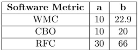
software metrics in the data set, we have used the findings of a systematic literature review conducted on 106 papers [89], which studies the applicability of 19 different software metrics for the task of software fault prediction. Out of the metrics reported by the study as having a strong positive effectiveness on software fault prediction, three can be found in our data sets, so we have decided to eliminate the other metrics. The metrics kept after the preprocessing are: WMC, CBO and RFC.
In order to build the fuzzy sets for the selected software metrics, we have taken inspira- tion from the work of Fil´o et al. [96]. They have used 111 software systems written in Java and computed the value of 17 different software metrics for each class of the systems. For each metric they have identifies thresholds to group the value of the metric in three ranges:
Good/Common, Regular/Casual, andBad/Uncommon. The threshold between the first two ranges was computed as the 70 percentile of the data, while the second threshold was consid- ered at the 90 percentile. Since the study presented in [96] contains thresholds for only one of the software metrics that we are using, we have decided to compute our own thresholds.
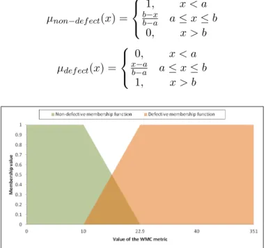
We have taken all data sets from the Tera-Promise repository [31] that belong to the Defectcategory and use the same software metrics as the data sets used for the experimental evaluation. In case of data sets with multiple versions, we have taken the last version. In this way, we have built a data set containing 6082 instances coming from a total of 30 projects. We have computed the 70 and 90 percentile for the metrics and used these values as thresholds for building two trapezoidal membership functions for thenon-defect anddefect classes. The first function measures the membership of a given software metric value to the class of non- defective entities, while the second one measures the membership to the class of defective entities. The two fuzzy membership functions for the WMC software metric are illustrated on Figure 2.9. Formulae 2.3 and 2.4 describe the equations used to compute the membership degree of a software metric value to thenon-defect, respectivelydefect fuzzy sets. The exact threshold values used for all three metrics are presented in Table 2.4.
µnon−def ect(x) =
1, x < a
b−x
b−a a≤x≤b 0, x > b
(2.3)
µdef ect(x) =
0, x < a
x−a
b−a a≤x≤b 1, x > b
(2.4)
Figure 2.9: Fuzzy membership functions for the WMC software metric.
2.2.3.2 Training
During the training process the fuzzy decision tree is built from the data set that was prepro- cessed as presented in the previous section. Defect detection data sets are usually imbalanced,
Software Metric a b
WMC 10 22.9
CBO 10 20
RFC 30 66
Table 2.4: Threshold values used to build the fuzzy membership functions for the used software metrics.
which can influence the training process and lead to afuzzy decision tree where each leaf node predicts that the given instance is non-defective. In order to reduce the imbalance of the data set, we enhance it before the training process, by adding extra defective instances from other data sets. These instances are used only for the training process, they are not considered during the testing.
Building thefuzzy decision tree (FuzzyDT)
The building process for the fuzzy decision tree proposed in the current paper resembles the one for a crisp variant of a decision tree with several alterations to cope with uncertainty and data imbalance. Both of these aspects have an important effect on the proposed fuzzy decision tree version shaping it into a custom variant tailored to solve the given problem as accurately as possible.
In order to manage the uncertainty of software defect prediction the defective and non- defective concepts needed to be formalized as fuzzy sets with respect to each of the attributes inside the data set. The method of fuzzy set construction for both of the target classes was presented in the previous section, but it must be added that an intensive selection process was necessary to highlight the attributes that may have a beneficial impact on the fuzzy decision process as many attributes in the data set were naturally not suited to aid any form of clas- sification. This is an aspect that contributes to the difficulty of the defective/ non-defective classification task. It must be mentioned that in order for the fuzzy approach to work, the fuzzy membership functions employed in the decision process need to be handled very del- icately preferably their devise being the fruit of a collaboration with software engineering experts. If the fuzzy membership functions do not map accordingly onto real contexts, the whole decisional process will be affected.
Once the fuzzy membership functions are constructed for each attribute, separately on each target class, the real fuzzy decision tree construction may commence. At this point, the other major problem discussed in the introduction occurs: data imbalance. Due to the scarceness of defective instances, the defective target class will be clearly imbalanced with respect to the non-defective target class on the studied attributes. In the classic fuzzy decision tree approach, the fuzzy entropy and fuzzy information gain measures are very biased with respect to data imbalance and this impacts the decision process in the sense that there is a clear inclination towards labeling instances as non-defective simply because the training set contains a significantly increased number of non-defective instances. This is an important issue with deep implications in the decisional process and therefore finding a way to deal with data imbalance was imperiously necessary.
A solution to the imbalance problem was proposed in [64]. Instead of choosing to follow other rather simplistic approaches that directly affect the data set such as over-sampling or under-sampling, which in our opinion are not fit for the present problem because the discrepancy between defective and non-defective instances is too high, the authors propose a way of coping with the imbalance by transforming the entropy and information gain measures.
In this way, from a constructional point of view, the only alteration will be changing the entropy and information gain formulae to a form that takes the imbalance into account and includes it in the computation, therefore attenuating its impact. Let us consider, in the
following, that thedefectiveclass is thepositiveone and thenon-defective class is thenegative one. As we have mentioned in Section 2.2.2.1, each internal node from the tree stores all the instances from the training data setD, but each instance has a certain membership degree.
The entropy measure at a node from the fuzzy tree is computed as in Formula (2.5) and generalizes theentropy computation from the crisp case.
Entropy(node) =−m+
mm·log m+
mm− m−
mm·log m−
mm (2.5)
wherem+ represents the sum of the membership degrees for the instances fromDbelonging to the positive class, m− sums the membership degrees for the instances from D belonging to thenegative class andmmis the sum of m+ and m−.
For computing theinformation gain of an attributeawith respect to the set of instances stored at an internal nodenodefrom thefuzzy tree, a kind of confusion matrix at that node is computed. We denote byF+a and F−a thefuzzy functions associated to attribute aand to thepositive and negative class, respectively. ByT PF uzzy,F PF uzzy andF NF uzzy we express the values which generalize (for thefuzzy case) the components of the confusion matrix for the crisp case. More exactly, these values are computed as follows:
• T PF uzzy sums the membership degrees for the instances i belonging to the positive class multiplied with the result of applying the function F+a on the value of attributea in instance i.
• F NF uzzy sums the membership degrees for the instances i belonging to the positive class multiplied with the result of applying the function F−a on the value of attributea in instance i.
• T NF uzzy sums the membership degrees for the instances i belonging to the negative class multiplied with the result of applying the function F−a on the value of attributea in instance i.
• F PF uzzy sums the membership degrees for the instances i belonging to the negative class multiplied with the result of applying the function F+a on the value of attributea in instance i.
We use the following notations:
• m=T PF uzzy+T NF uzzy +F PF uzzy +F NF uzzy.
• p=T PF uzzy+F NF uzzy.
• pp=T PF uzzy+F PF uzzy.
Using the previous notations, the new formula for the information gain measure is pre- sented in Formula (2.6).
IG(node) =Entropy(node)− pp
m ·E1− m−pp
m ·E2 (2.6)
where
E1 =−T PF uzzy
pp ·logT PF uzzy
pp −F PF uzzy
pp ·logF PF uzzy pp and
E2=−T NF uzzy
m−pp ·logT NF uzzy
m−pp − F NF uzzy
m−pp ·logF NF uzzy m−pp .
2.2.4 Testing
After thefuzzy decision tree was trained (as described in Section 2.2.3.2), a new instance will be classified as shown in Section 2.2.2.1.
For evaluating the overall performance of the FuzzyDT model, a leave-one out cross- validation is used [110]. In the leave-one out (LOO) cross-validation on a data set with n software entities, theFuzzyDT model is trained onn-1 entities and then the obtained model is tested on the instance which was left out. This is repeatedn times, for each entity from the data set.
During the cross-validation process, the confusion matrix [87] for the two possible out- comes (non-defect anddefect) is computed. We are considering that thedefectiveclass is the positive one and thenon-defective class is the negative one. The confusion matrix contains four values, the number ofTrue Positives (T P),True Negatives (T N),False Positives (F P) andFalse Negatives (F N). For computing the values from the confusion matrix, we are using the known labels (classes) for the training instances.
Since the software defect prediction data are highly imbalanced (the number ofdefects is much smaller than the number ofnon-defects) the main challenge in software defect prediction is to obtain a largetrue positive rate and a small false negative rate. For defect predictors, theaccuracy of the classifier (i.e. number of testing instances which were correctly classified - Formula (2.7)), is not a relevant evaluation measure, since the imbalanced nature of the data.
Acc= T P +T N
T P +T N +F P +F N (2.7)
A more relevant evaluation measure for the performance of the software defect classifiers is theArea Under the ROC Curve (AUC)measure [36] (larger AUC values indicate better defect predictors). The AUC measure is usually used in case of approaches that output a single value which is transformed into a class label using a threshold. For such approaches, modifying the value of the threshold can lead to different values of theProbability of detection (Formula (2.8)) and the Probability of false alarm (Formula (2.9)) measures. For each threshold, the point (P f,P d) is represented on a plot, and AUC measures the area under this curve.
P d= T P
T P +F N (2.8)
P f = F P
F P +T N (2.9)
In case of approaches where the output is directly the class label, there is only one (P f, P d) point, which can be linked to the (0,0) and (1,1) points, and the area under this curve can be computed using Formula (2.10).
AU C = (1−P f)∗P d+P f∗P d
2 +(1−P f)∗(1−P d)
2 (2.10)
2.2.5 Experimental evaluation
In this section we provide an experimental evaluation of the FuzzyDT model (described in Section 2.2.3) on two open-source software systems which were previously used in the software defect prediction literature. We mention that we have used our own implementation for FuzzyDT, without using any third party libraries.