The papers in this volume were presented at the 22nd International Conference on Principles of Distributed Systems (OPODIS 2018), held in December in Hong Kong, China. All aspects of distributed systems are within the scope of OPODIS: theory, specification, design, performance and system construction.
Program Committee
General Chair
Program Chairs
Corentin Travers, University of Bordeaux, France Jennifer Welch, Texas A&M University, USA Josef Widder, Technische Universität Wien, Austria Yongluan Zhou, University of Copenhagen, Denmark.
Steering Committee
Organization Committee
List of Authors
Graduate Studies in Information Science and Technology, Osaka University, Japan kakugawa@ist.osaka-u.ac.jp. Graduate Studies in Information Science and Technology, Osaka University, Japan masuzawa@ist.osaka-u.ac.jp.
Sparse Matrix Multiplication and Triangle Listing in the Congested Clique Model
Keren Censor-Hillel
Dean Leitersdorf
Elia Turner
1 Introduction
- Our contribution
- Challenges and Our Techniques
- Related work
- Preliminaries
As defined earlier, for a matrix Awe bynz(A) denotes the number of non-zero elements of A. Throughout the paper we must also refer to the number of non-zero elements in certain submatrices or sequences.
2 Fast Sparse Matrix Multiplication
Fast General Sparse Matrix Multiplication - Algorithm SMM
With this information, the nodes locally compute the n-partitioned pair (a, b) that minimizes the expressionnz(S)·b/n2+nz(T)·a/n2+n/ab, which describes the round complexities of each of the three parts of Algorithm SBMM. Finally, in the last loop, nodev receives the row v ofP =A−1σ P0A−1τ, which completes the correctness of the algorithm SMM.
Fast Sparse Balanced Matrix Multiplication - Algorithm SBMM
Thus, all nodes in line 9 can agree on the assignment of the subsequences, where each node is assigned at most 2 subsequences of entries of S and 2 of entries of T. At the end of the execution of Compute-Sending in Algorithm 4, we have each node v at most two subsequences in BS(v) and at most two subsequences in BT(v).
3 Discussion
In Proceedings of the Twenty-6th Annual ACM-SIAM Symposium on Discrete Algorithms (SODA), pages. Increasing the efficiency of sparse matrix-matrix multiplication with a 2.5D algorithm and one-sided MPI.CoRR, abs.
Large-Scale Distributed Algorithms for Facility Location with Outliers
Tanmay Inamdar
Shreyas Pai
Pemmaraju
Main Results
The first contribution of this paper is to show that O(1) approximation algorithms to RobustFacLocand FacLocwith Penalties can also be obtained using variants of the Mettu-Plaxton greedy algorithm. Our second contribution is to show that by combining ideas from earlier work [21, 4] with some new ideas, we can efficiently implement distributed versions of the variants of the Mettu-Plaxton algorithm for RobustFacLocandFacLoc with Penalties.
2 Sequential Algorithms for Facility Location with Outliers
Robust Facility Location
We begin by assuming that we get a facility, e.g. with opening cost fie, such that,fi∗≤fie ≤αfi∗, where α≥1 is a constant. Note that we can remove the facilities with opening costs +∞ without affecting the price of an optimal solution, and therefore we assume that w.l.o.g.
Facility Location with Penalties
This algorithm can be thought of as running O(logn) separate instances of a modified version of the original Mettu-Plaxton algorithm (Algorithm 1), where in each instance of the Mettu-Plaxton algorithm, the algorithm terminates as soon as the number of clients falls below the required number, followed by some post-processing. We slightly abuse the notation and use (C0, F0) to denote the solution returned by the algorithm, i.e. solution (Ct0, Ft0) corresponding to the iteration of the outer loop that results in the minimum cost solution.
3 Distributed Robust Facility Location: Implicit Metric
The k-Machine Algorithm
Again, as in the analysis of the sequential algorithm, we abuse the notation so that (i) (C0, F0) refers to the minimum-cost solution returned by the algorithm, (ii) refers to the option chosen in line 2 of the algorithm, and (iii) modified copy with original installation costs. This analysis appears in the full version [24] and as a result we obtain the following theorem.
The Congested Clique and MPC Algorithms
Therefore, all we need to do is to efficiently implement an approximate SSSP algorithm in the MPC model. 6] provide a distributed implementation of their approximate SSSP algorithm in the Broadcast Congested Clique (BCC) model.
4 Distributed Robust Facility Location: Explicit Metric
The Congested Clique Algorithm
The MPC Algorithm
5 Conclusion and Open Questions
In Proceedings of the 18th Annual ACM Symposium on Parallelism in Algorithms and Architectures (SPAA), pp. In Proceedings of the 30th Annual ACM Symposium on Principles of Distributed Computing (PODC), pp.
Equilibria of Games in Networks for Local Tasks
Paolo Penna
Motivation and Objective
- Locally Checkable Labelings
- A Generic “Luby’s Style” Randomized Algorithm for LCL Tasks
- LCL Games
Then v chooses a random temporary label, tmp-label(v), compatible with the current fixed labels of the nodes in the observed ball. A strategy for a node: a probability distribution. Use the labels compatible with the ball of radius t, centered atv, which may depend on the history of v during the execution of the generic algorithm.
Our Results
The payoff function πv of node v at the completion of the algorithm decays with the number of rounds before the algorithm terminates atv. The rest of the paper therefore focuses on the formalization of LCL games, and on the proof of Lemma 3.
Related Work
The most interesting part of the proof, in terms of local distributed computing on networks, is to show that LCL games satisfy all the requirements defined in Lemma 2. Many games on networks have complete information and, among games with incomplete information , a large part of the literature is devoted to one-stage games where the players are initially unaware of the network topology (see survey [18]).

2 The Extensive Games Related to LCL Games
- Basic Definitions
- Well-Rounded Games
- Strategies, Outcomes, and Expected Payoff
- Equilibria, and Subgame Perfection
- Metrics
- Equilibria of Extensive Games Related to LCL Games
Note that each component of the expected payoff function is bounded by M, where M is the upper bound of each payoff. Finally, we define the continuity of the expected payoff function using the sup overRn norm.
3 Proof of Lemma 3
Formal Definition of LCL Games
From now on, the players are identified by the vertices of the graph G, labeled from 1 to n. We define the end time of the player's history zbytimei(z) = max{|actionsj(z)|, j∈ball(i)} −1. The game's payoff function π is then defined as follows.
The proof of Lemma 3
Since xandy are in the same information set, it follows that for each player j ∈ ball(i) we have actionj(x) = actionj(y). We have timei(z) 4 Conclusion and Further Work The Sparsest Additive Spanner via Multiple Weighted BFS Trees Ami Paz Thus, we introduce a new sequential algorithm to the problem and then present its distributed implementation. Another approach to the distributed construction of (+6) keys could be to adapt a distributed algorithm with different stretch guarantees to construct a (+6) key. Prime examples for the need for sparse keys can be found in distributed network synchronization [42], information distribution [9], compact routing schemes, and more. This lower bound does not take into account bandwidth limitations at all (it has been proven for the local model), and so we believe that a higher lower bound should apply to the contention model, but this is left as an open question intriguing. J Lemma 6 implies that as the algorithm progresses, messages are sent and updated at higher indices of the proximity list. This lemma states that a truncated list is correct at the beginning of the corresponding round. According to Lemma 5, there is a roundr0 when all entries of PL(rv0) are correct, and let (ds, s, ws) be a triplet in one of the first minutes. According to Lemma 6(i), when the triplet is inserted into the list, it is already placed in one of the first minutes. By summing over allO(logn) values of k, and adding the number of edges contributed by the cluster phase, we conclude that H has at most. Therefore, k0, the number of edges inσ\H0, is less than the number of clustered nodes inσ. 13 Atish Das Sarma, Stephan Holzer, Liah Kor, Amos Korman, Danupon Nanongkai, Gopal Pandurangan, David Peleg dan Roger Wattenhofer. The Amortized Analysis of a Non-blocking Chromatic Tree Our amortized analysis for the chromatic tree is based on the amortized analysis for the unbalanced binary search tree by Ellen, Fatourou, Helga and Ruppert [7]. In section 3, we provide an overview of related work done on the amortized analysis of concurrent data structures. The amortized step complexity of a data structure is the maximum number of steps in any execution consisting of operations on the data structure, divided by the number of operations called in the execution. For an operation on an executionα, we define itspoint contentionc(op) as the maximum number of active operations in a single configuration˙ during the execution interval from op. In the initial configuration, the data structure represents an empty instance of the abstract data type and there are no active operations. One can determine an upper bound on the amortized step complexity by assigning an amortized cost to each operation, such that for all possible executionsαon the data structure, the total number of steps taken inα is at most the sum of the amortized cost of the operations inα. At this point, the inR nodes are no longer reachable from the root of the chromatic tree. Consequently, we will consider an implementation of the chromatic tree using a stack to recover from failed attempts. In this section, we count the number of cleanup attempts that fail due to failed LLXs. The total number of dollars deposited into the bank by an operation is O(h(cp) +rebal(viol(cp))·c(cp))˙ during its cleanup phasecp. Consider a failed attempt from cp due to a failed LLX during a non-stale instance of TryRebalance. According to rule W-L, a failed LLX(x) can instead withdraw a dollar from Bllx(cp, p), where pisses the parent ofx. A successful CAS freeze at a node below xof an SCX reduces H(x) by 1 and does not increase H(u) for any other node in the chromatic tree. By Lemma 21.5, a commit step increases H(x) by at most 1, for all nodes x in the chromatic tree. J Since all bank accounts owned by cphave non-negative balance, Property P3 of the bank is satisfied. Lock-Free Search Data Structures: Throughput Modeling with Poisson Processes Aras Atalar Paul Renaud-Goud In order to estimate the delay of the events, the errors, which are sensitive to the overlap of these events in the timeline, must be taken into account. On the other hand, coherency cache misses arise due to modifications, often performed with Compare-and-Swap (CAS) instructions, to the lock-free lookup data structure. Knowing the probabilistic order of these events provides crucial information used in estimating the access delay associated with a triggered event. In [12, 24], various performance shapers for randomized trees, such as the time complexity of operations, expectation, and depth distribution of nodes based on their keys, are studied. On the other hand, several performance measures for search data structures have been studied for the sequential setting. Algorithm parameters: Expected latency of the application-specific code (interlacing data structure operations) tapping, local computation cost while accessing a nodetcmp (a constant cost of a few cycles for the key comparisons, local updates for cursor chasing), probability mass -functions for the key and operation selection. For a given nodeNi, we denote byλacci (resp. λreadi, λcasi) the rate of events that cause an access (to quantify the error in approximations of the Poisson process, we derive experimentally the cumulative distribution function of the delay between the arrival of events that occur at a given node. Note that the search data structures generally contain several sentinel nodes that define the boundaries of the structure and are never removed from the structure: their presence probability is 1. In particular, this implies that the access trigger events follow a Poisson process with rate λacci =λreadi +λcasi , and that the read-trigger events originating from P0 different wires and occurring at Ni follow a Poisson process with rate P0×λreadi. Solving Process It remains to combine these access latencies to obtain the throughput of the search data structure. The equation applies to every node in the query data structure, and to the application call that occurs between query data structure operations. Similarly, we calculate the access probability of the internal node with keyk in an operation targeting keyk0. The number of internal nodes in the interval [k, k0] (or (k0, k] if k0 < k) is actually a random variable, which is the sum of independent Bernoulli random variables that model the presence of the nodes. We define the reading speedλreadint,k,h of these virtual nodes as a weighted sum of the initial speed of the nodes thanks to the two equations pintk =PHk. More details can be found in [4], how to get the mass function of the random variableSubk to calculate read rates for virtual nodes and how to deal with CAS events. For the data structure implementations, we have used ASCYLIB library [11] coupled with an epoch-based memory management mechanism which has negligible latency. 8 Conclusion Concurrent Robin Hood Hashing Robert Kelly Barak A. Pearlmutter Hash tables are one of the key building blocks in software applications, providing efficient implementations for the abstract map and array data types. Robin Hood Hashing [7] is an open-address hash table method in which entries in the table are shifted so that the variance of the distances to their original bucket is minimized. As can be seen, the entry gets much further away using Linear Probing than using Robin Hood. In Robin Hood, however, the DFB of the entry is important, as subsequent lookups use this metric to determine whether the entry being queried is contained in the table. Logical deletion is unacceptable as it causes the table to fill up and lose its efficiency, resulting in unnecessary resizing. Backward shift effectively undoes the insertion of the record we want to delete from the table. If a discrepancy is found, the search is restarted, otherwise we know for sure that the key is not in the table. If the key is not found, as per Contains, timestamps are checked in case a concurrent RemoveorAdd moved the key during the search. Experimental Setup The cache results are shown in Table 1 as a percentage against K-CAS Robin Hood for a single core. The lower occupancy rate shows that K-CAS Robin Hood is slightly beaten by the Transactional Robin Hood. All workloads show that the gap between K-CAS Robin Hood and Hopscotch starts to narrow once HyperThreading™. Maged Michael scales well on tested workloads, although the line gradient is not steep enough to challenge K-CAS Robin Hood or Hopscotch Hashing. Proceedings of the International Conference on High Performance Computing, Networking, Storage and Analysis, SC. Parallel Combining: Benefits of Explicit Synchronization Petr Kuznetsov One of the processes with an active request becomes a combiner and batches the requests in the set. Under the coordination of the combiner, the owners of the collected requests, called clients, apply the requests in the batch to the parallel batched data structure. Our performance analysis shows that implementations based on parallel combination can outperform state-of-the-art algorithms. But clustered implementations can also use parallelism to speed up cluster execution: we call these clustered parallel implementations. Unlike the classic PRAM model, each process executes its instructions independently of the timing of the other processors. Then selects one of the completed successors to execute and adds the remaining completed successors to the bottom of its deque. STATUS_SET contains, by default, the values INITIAL and FINISHED: INITIAL which means that the request is in the initial state and FINISHED which means that the request has been served. Parallel Batched Algorithms Each read-only operation is linearized at the point where the combiner sets the state of the corresponding request to STARTED. By the algorithm, a read-only operation observes all update operations applied before and during the current combine phase. If the combiner's request is ExtractMin, it also executes the above code as a client. Otherwise, the combinerCountry inR– calculates the number of target nodes in the left and right subtree ofv. This algorithm works in O(logm+clogc) steps (and can be optimized to O(logm+c) steps), where is the size of the queue and is the number of Insert requests to be used. For further details on the parallel algorithm, we refer to the full version of the paper [3]. So the plot for RWLock is almost flat, it gets a little worse as the number of processes increases, and we blame traffic for that. As the number of processes increases, the synchronization cost increases significantly for all algorithms (in addition to FC Binary and FC Pairing not being able to scale). The main drawback of this approach is that all processes must perform CAS at the top of the list. A process with a task to perform on the data structure stores it in the request pool and attempts to obtain a global lock. They provide provable bounds on the running time of a multithreaded dynamic parallel program, using P processes and a specified scheduler. As shown in Section 6, our concurrent priority queues perform well compared to state-of-the-art algorithms. Specification and Implementation of Replicated List: The Jupiter Protocol Revisited Hengfeng Wei Each client maintains a single state space that is synchronized with the states of other clients through a counter state space maintained by the server. CJupiter is compact in the sense that, at a high level, it maintains only a single ordered state space that contains exactly all the states of each replica. We adopt the convergence property in [5], which requires that two Read operations observing the same set of list updates return the same response. This is allowed by specifying the weak list with list ordering lo: b−lo→aon w1, a−lo→xonw2, andx−lo→bonw3. Data Structure: n-ary Ordered State Space First, the sequence of operations along the first edges from a vertex of the CSSsat server admits a simple characterization. Consider the CSSat server shown in Figure 4 under the plan of Figure 1; see Figure B.1a of [25] for its construction. CJupiter is Compact When clientci receives an operation op∈Op from the server, it transforms with an operation sequence along the local dimension in its 2D state space DSSci to obtain opp0 by calling xForm(op,LOCAL) (see below), and applies op0 locally. Figure 6 (Rotated) illustration of client c3, as well as the servers, in Jupiter [26] under the schedule of Figure 1. Suppose that under the same schedule, the server has processed a sequence of operations, denoted O=hop1,op2,. Under the same schedule, the behavior (ie the sequence of (list) state transitions, defined in section 2.1) of the servers in CJupiter and Jupiter is the same. The Clients Established Equivalent Under the same schedule, the behavior (i.e. the order of (list of) state transitions, defined in Section 2.1) of the servers in CJupiter and Jupiter is the same. . 12:14 Replicated List Specification and Implementation: The Jupiter Protocol Revisited. Letv0 is the unique LCA of a pair of vertices v1 and v2 in the n-ary ordered state space CSSs, denoted v0=LCA(v1, v2). 6 Related Work I Proceedings of the 8th Annual ACM Symposium on User Interface and Software Technology, UIST ’95, side 111–. InProceedings of the 13th International Conference on Stabilization, Safety and Security of Distributed Systems, SSS'11, side 386-400. Local Fast Segment Rerouting on Hypercubes Klaus-Tycho Foerster Stefan Schmid This is problematic as certain applications, e.g. in data centers, is known to require a latency of less than 100 ms [67]; voice traffic [33] and interactive services [35] degrade already after 60 ms delay. All routing rules must be precomputed and must not be changed at runtime (eg after errors). We only allow routing rules that match 1) the packet's next destination (ie the top of the label stack)2 and 2) event link failure.3 When a packet hits a failed link`= (u, v) at some nodeu, the current nodeum can push a set of pre-calculated labels on top of the current label stack, to create a so-called backup path tow (which can also be traversed in reverse from tou). In the following, we'll explore backup path schemes that guarantee packet delivery even with multiple failures. In the next section, we will show how to efficiently generate a (k−1)-resilient backup path scheme for k-dimensional hypercubes. A mixed chain is the aggregation of multiple chains (across multiple dimensions) that cross each other sequentially. In other words, a mixed chain consists of chains of links in at least two dimensions. First, we show that for everyd∈[k] every cycle of dependence over d-dim links is at least k long. Therefore, R=long is sufficient to ensure the length of any dependency cycle caused by d-dim connections, 2R≥k. To show that the scheme is (k-1)-resistant, we claim that each dependency cycle consists of at least clicks. The combination of (1), (2), and (3) implies that there must be at least k dependencies in the assumed dependency cycle, which concludes our claim. 0 is on the shortest path from the tail of `0 rope, therefore on the backup path. Given a possible assignment, the value of everydxy is at most the length of the shortest path fraxtoy. The length of the shortest cycle of dependencies through each dependency arc (`1, `2) is bounded by (11). PMSR—Poor Man's Segment Routing, a minimalist approach to Segment Routing and a Traffic Engineering use case. Effects of Topology Knowledge and Relay Depth on Asynchronous Appoximate Consensus Dimitris Sakavalas Limited topology knowledge and relay depth (section 3): We consider the case of k-hop topology knowledge and relay depth depth. Topology detection and unlimited relay depth (section 4): We consider the case with one-hop topology knowledge and relay depth n. Extensive previous works have studied graph properties for other similar problems in the presence of Byzantine faults, such as (i) Byzantine approximate consensus when using directed graphs. The following theorem presented in [23] states that the CCA (Crash-Consensus- Asynchronous) condition is tight for approximate consensus in complete knowledge of topology and relay depth. The lemma below states that the interval to which the states at all the fault-free nodes are bounded shrinks to a finite number of phases of Algorithm LocWA. The theorem is then proved using simple algebra and the fact that the interval to which the states of all the fault-free nodes are restricted shrinks to a finite number of phases. For Fi ⊆Ni−(k) reachki(Fi) denotes the set of nodes that have paths of length 1≤k to nodeiinGV−Fi. After defining the basic notion in (A → k B), definition 6 of the notion A propagates to Bis the same for the case of k-hop. Condition Relation and Convergence Time Comparison Condition Relation Convergence Time Comparison This is why the LWA Algorithm allows each node to learn enough state values to reach rough consensus. The LWA algorithm also works on undirected graphs, as shown in the full version [21]. On the other hand, in an execution of Algorithm 2-LocWA, nodeD will only receive a message from C in one round, since (C, B) is a directed edge and delay on edges (A, C) and (B, D ) ice in this case, D will not be able to decide before the round, the first round in which condition 2-WAIT will be satisfied. As shown in the full version [21], the thek-WAIT mode fork-LocWA algorithm can be strengthened such that fork0≥can and any, Algorithmk0-LocWA will converge faster than Algorithmk-LocWA. Hybrid Fault-Tolerant Consensus in Asynchronous and Wireless Embedded Systems Wenbo Xu Signe Rüsch Bijun LiNoam Ravid
Other spanner construction algorithms
2 Preliminaries
3 Multiple Weighted BFS Trees
4 A (+6)-Spanner Construction
Algorithm 6AP

5 Discussion and Open Questions
Jeremy Ko
2 Model
3 Related Amortized Analyses of Non-blocking Data Structures
4 The Non-blocking Implementation of the Chromatic Tree
An Implementation of a Chromatic Tree using LLX and SCX

5 Chromatic Tree Amortized Analysis
Bounding the Number of Failed Cleanup Attempts
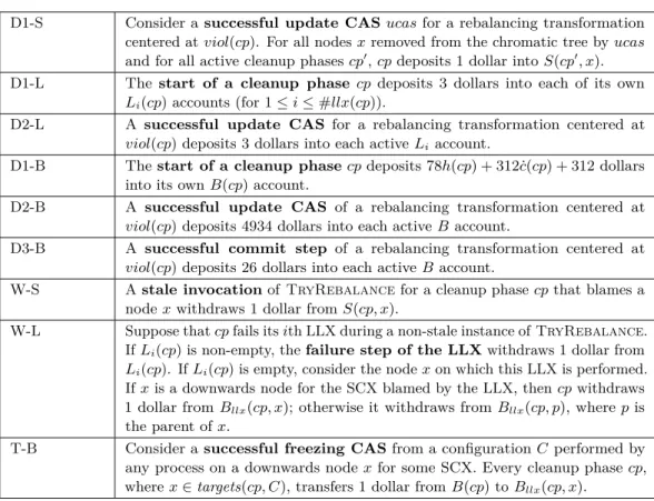

The B(cp) Accounts
6 Conclusion
Philippas Tsigas
2 Related Work
3 Problem Statement
4 Framework
Event Distributions
Impacting Factors
5 Throughput Estimation 5.1 Access Latency
Latency vs. Throughput
6 Instantiating the Throughput Model
7 Experimental Evaluation
Setting
Search Data Structures
Phil Maguire
2 Background 2.1 Prior Work
Original Robin Hood

K-CAS
3 Algorithm

4 Performance, Results, and Discussion
Discussion and results

Future Work
5 Conclusion
Anatoly Shalyto

2 Background
3 Parallel Combining
Combining Data Structure
Specifying Parameters
4 Read-Optimized Concurrent Data Structures
5 Priority Queue
6 Experiments
Concurrent Dynamic Graph

Priority Queue
7 Related Work
8 Concluding remarks
Jian Lu
2 Preliminaries: Replicated List and Operational Transformation
3 The CJupiter Protocol
The CJupiter Protocol

4 CJupiter is Equivalent to Jupiter
Review of Jupiter
The Servers Established Equivalent
5 CJupiter Satisfies the Weak List Specification
7 Conclusion and Future Work
Tao Wen

3 Efficient Resilient Segment Routing on k-Dimensional Hypercubes
Overview of the Fast Local Failover Scheme
Proof Preliminaries
Correctness
4 Related Work
5 Conclusion and Future Work
Future Work I: Resilient Segment Routing on General Graphs
Future Work II: Testbeds for Fast Failover in Segment Routing

Lewis Tseng

2 Preliminary
3 Limited Topology Knowledge and Relay Depth
General k Case
4 Topology Discovery and Unlimited Relay Depth
5 Discussion


