Raimund Seidel (Universität des Saarlandes und Schloss Dagstuhl – Leibniz-Zentrum für Informatik) Thomas Schwentick (TU Dortmund). Dieser Band enthält die Beiträge und ausführlichen Zusammenfassungen der eingeladenen Vorträge, die auf der Konferenz gehalten wurden.
Justified Representation in Multiwinner Voting
Edith Elkind
1 Setup
However, in our example this means that the chair will end up choosing four candidates who only appeal to "Theory A" (i.e. algorithms and complexity) researchers, and this does not seem fair: if there are four invited talks, and the formal method community is represented by 9 = 36/4 PC members, intuitively the formal methods researchers are entitled to at least one slot (which they probably want to assign to candidateF). On the other hand, it seems that at least two slots should go to "Theory A" speakers, since they are supported by more than half of the voters.
2 Formal Model
Examples of Committee Selection Rules
In what follows, we will examine recent research that contributes to our understanding of such scenarios by proposing appropriate axioms and identifying voting rules that satisfy them; we will also discuss the computational complexity of the associated problems.
Elkind 1:3
Rules based on fractional vote transfers One problem with the GrMonAV rule is that it matches each voter to a single alternative; if a voter does not approve of the alternative she is suited to, of course we cannot expect her to be satisfied with the chosen committee. Just as for PAV, finding optimal committees under this rule is NP-hard [8], and Phragmén developed an iterative version of this rule, which is computationally tractable (again long before the concept of computational complexity was formalized); the subsequent literature [16] refers to this rule as SeqPhragmen.
3 Axioms
Elkind 1:5
A committee W provides extended justifiable representation (EJR) if for every `∈[k] and every `-large,`-coherent group of votersV, there exists an elector∈V that approves at least`members ofW, i.e. |Ai∩W |. A committee W provides proportional justifiable representation (PJR) if for every ` ∈ [k] and every `-large, `-coherent group of voters V, there are at least ` members of W approved by a voter from V, i.e. .
Elkind 1:7
4 Algorithms
In contrast, creating an effective process for finding committees that provide EJR has proven to be more challenging. Recently, three manuscripts providing polynomial-time procedures for computational committees providing EJR and a manuscript demonstrating conP-completeness for testing whether a given committee provides PJR were combined into a paper accepted at AAAI-18 [2].
5 Conclusions
Elkind 1:9
A Markov Chain Theory Approach to
Characterizing the Minimax Optimality of
Stochastic Gradient Descent (for Least Squares)
1 Introduction
This work provides a brief proof of this minimax optimality for SGD for the special case of least squares through a characterization of SGD as a stochastic process. For the case of additive noise models (i.e. the “well specified” case) the assumption is that y=w∗·x+η, where η is independent of x).
2 Statistical Risk Bounds
In the incorrectly specified case, an example from [5] shows that such a smaller step size is needed to stay within a constant factor of the minimax rate. An even smaller step size leads to a constant that is even closer to that of the optimal speed.
3 Analysis
The Bias-Variance Decomposition
The bias term (the first term) decays at a geometric rate (one can set = T /2 or maintain multiple running averages if T is not known in advance). The bias term is characterized as follows: it applies because wt−w∗means 0 and both xt+1 and ξt+1 are independent ofwt−w∗).
Stationary Distribution Analysis
Also note that for PSD matrices A, B, TrAB≥0. and the series converges because I−γH≺I. 2:8 A Markov chain approach to show the minimum optimality of SGD for least squares. The inverse of this operator can be written as: which exists since the sum converges due to that 0I−γHI.
Completing the proof of Theorem 1
Automated Synthesis: a Distributed Viewpoint
Anca Muscholl
1 Overview
Runtime verification is an attractive alternative method to traditional exhaustive exploration, situated somewhere between testing and model checking (see e.g. the surveys [12, 10] and the dedicated conference RV running for more than 15 years). The reactive synthesis of distributed programs is a particularly attractive problem because distributed programs are notoriously difficult to get right.
2 Going distributed
Muscholl 3:3
The decidability status of reactive distributed synthesis in this model is still open, but the problem is known to be decidable when the communication structure is acyclic [8, 16]. The synthesis problem was shown to be solvable when there is a single environment token and a limited number of system tokens [4].
Muscholl 3:5
Matrix Estimation, Latent Variable Model and Collaborative Filtering ∗†
Devavrat Shah
Model, Problem Statement
Let F be an n×n matrix that we would like to estimate, and let Z be a noisy signal of matrixF such that E[Z] = F. We must assume that the expected data matrix can be described by the latent function f, i.e.
Related Works
We will assume that each u∈[n] is associated with a latent variable αu∈ X1, which is drawn independently through the indices [n] according to the distribution P1 over a bounded compact space X1. For each observation, we assume that E[Z(u, v)] =F(u, v),Z(u, v) is bounded and {Z(u, v)}1≤u These recent results suggest that the practical success of these methods in various applications may be due to their ability to capture local structure. A key limitation of this approach that this work overcomes is the ability to handle sparsity. Distance using Immediate Neighbors Distance using Far-away Neighbors Shah 4:5 Distance Using Immediate Neighbors Distance Using Immediate Neighbors Shah 4:7 Some Open Problems in Information-Theoretic Cryptography Furthermore, all known approaches to theoretically secure computations have a communication cost that is proportional to the computational cost of the function (in some computational models, say as a Boolean or arithmetic circuit). It is worth noting here that a simple enumeration argument establishes the existence of functions that require exponentially large circuits, but a similar statement is not known for communication cost. In particular, in the case of 3 parties, the PIR protocol of [15] gives us a 3-party computation protocol for arbitrary functions with communication 2O(˜. √n), in which the total input size. In contrast, in the private environment we have a large gap between upper and lower limits. Proceedings of the 19th Annual ACM Symposium on Theory of Computing, 1987, New York, New York, USA, pages 218–. InAdvances in Cryptology – EUROCRYPT 2004, International Conference on Theory and Applications of Cryptographic Techniques, Interlaken, Switzerland, May Proceedings, p. Vaikuntanathan 5:7 Backward Deterministic Büchi Automata on Infinite Words Thomas Wilke In other words, this automaton must be expanded to get back a deterministic Büchi automaton for the language in question. For every inverse deterministic generalized Büchi automaton with n states and mBüchi sets, there is an equivalent inverse deterministic Büchi automaton with 2mn states (even if the transition conditions are used in the generalized Büchi condition, that is, if B ⊆2S×A×S). The proof of the second claim is an example of the question of how to transform a backward deterministic generalized Büchi automaton into an equivalent backward deterministic automaton, because by a direct product construction, given two backward deterministic Büchi automata, one can a backward determinant is constructed. generalized Büchi automaton (with two Büchi groups) recognizing the intersection of known languages from the given automata. To conclude this section, we explain how the required semantic property can be checked by a deterministic backward automaton ω. For the other direction, from backward deterministic counterfree automata to future time formulas, an embedded inductive argument can be used, see [18]. An ω language can be expressed in future time logic if, and only if, it is recognized by a counter-free backward deterministic (generalized) Büchi automaton. A function Aω → {0,1}ω is expressible in the temporal logic of the future/past if and only if it is realized by a counter-free bimachine. The other direction follows from the fact that counter-free automata on finite words and backward deterministic counter-free Büchi automata define temporal properties. To show what the answer to one of the other questions looks like, we consider Fexpressibility - the second question. An ω-language recognized by a backward deterministic (generalized) Büchi automaton with inverse transition function δ can be defined in time logic if and only if the quotient transition function δ/≡ does not have one of the following patterns. A temporal property can be expressed in the F fragment of future time logic if, and only if, the following holds for every backward deterministic automaton of the ω language defined by the property. Note that the second pattern indicates that the property is stem-invariant: if an ω-word is the result of another ω-word by compressing or emptying chunks consisting of the same symbol, then either both words or neither are accepted them. Specifically, tacit events (or actions) are computational steps whose specific nature is not revealed at the abstraction level of the system model. It is even less clear to what extent tacit actions affect the monitorability of the relevant specifications. Nevertheless, the model still provides sufficient evidence of their manifestation during execution, which can play an important role in capturing vital behavioral aspects of the system: they can describe the branching structure of the modeled system behavior [20, 16] or provide a measure of computational cost and efficiency [4]. Properties of processes can be determined via µHML logic [18], a transformation of the modal µ-calculus [17]. We call the LTS monitor in Definition 4 Mδ, the entire instrumentation of Definition 5 Iδ, and the pair (Mδ, Iδ) as the entire control system. In the case of the (Mα, Iδ) monitoring system, the instrumentation more often forces the monitor to go into an indeterminate state as it does not deviate from the δ-transitions. Letmbe a monitor of a monitoring system (M, I);ϕ a formula of µHML on (Act,{τ});L an LTS on (Act,{τ}) – that is, L reports completely silent transitions ;. We say that reliably (M, I) monitors for ϕon Lifm (M, I) monitors for ϕon L of every eclipse ofL. Following Property 4.2, it is sufficient to require that it is reachable from pin L0 via a series of silent actions (Property 4.2). In Property 4.2 below, obfuscation can reach a point, represented as an LTSLo, where all the silent-action information is hidden. Furthermore, if a state is a sequence of silent transitions vL leading to a stateq that can perform an external action, then this observation must be stored in L0. We assume that there is a certain level of blackout above which adequate monitoring is impractical. The difference is that when the monitor expects a more obscure action (i.e. σ), the instrumentation can signal a potentially less obscure process action. As we will see in the following, we can further restrict the syntax of myopic monitors while maintaining controllability with respect to reliably checkable formulas. Ikonklusionmi babaen ti panangipalagip a dagiti myopic a monitor ket mabalin pay a mailadawan a kas ti pirgis dagiti naan-anay a monitor babaen ti panangsukat tiσ.nobyτ.no+σ.noandσ.α.mwithrex.(τ.x+σ.x+τ.α.m+σ .α .m) iti aniaman a myopic monitor. 12 Da Adrian Frankalanza, Luca Aceto, Antonis Achilleos, Duncan Paul Attard, Ian Cassar, Dario Della Monica ken Anna Ingolfsdottir. An up-contour (resp. down-contour) of a saddle point v is any contour of Mh(v)+ε (resp. A non-leaf node of R is called positive (resp. negative) if its corresponding saddle point is positive (resp. . negative). The figure shows the two possible ways in which (u, v1) and (u, v2) can map toR, and how it determines the changes in R. Note that in the presence of gender, there can be parallel arcs between a pair of nodes that undergo an exchange event. The operation LSCross(x, u) updates the cross level set(s) of x from intersecting down edges (up edges) at time t- to intersecting up edges (down edges) at time t+. LSCross(x, u) and Handoff(x, x0): For LSCross(x, u), our goal is to remove the edges of ufrom the intersection level of x one by one (assuming thath(x, t−)< h(u , t−) without loss of generality) using link-cut tree operations before adding the up-edges of utox's intersection level set. Additionally, we need to ensure that each edge still has copies of the intersection level array sorted by height. Finally, we call LSCross(v, u) ifv is now a proxy, because its (newly obtained) crossover level sets spend the excess time. Fα)-Deletion problem where at least two of the families are the family of all bipartite graphs is W[1]-hard. This problem assumes an odd cycle across the magnitude of most part of the input. Each instance of color OCTs is converted to a (G,P, O, k, `) polynomial-time instance of Color OCT Compression. Finally, for each instance of OCT color compression we generate 2O(k) instances of Color Separator, with parameterscand`≤αk, inO?(2O(k)) time. When k >0 and ∅ is a T-manifold cut, we can solve the corresponding instance in timeO?(2O(`)). If we can find a subset U ⊆ U that intersects all sets in F, such that|U| ≤k, then U is the required solution. The lemma is proved in a purely existential setting and serves as a proof of the correctness of the algorithm. Recall that Lemmas 3.1 and 3.2 together imply that if we can solve a Colorful Separator instance in O?(kpoly(α,k)) time, then the algorithm for simultaneous FVS/OCT follows. The jth copy of the vertex setVi will be used to ensure that there is an edge between the selected vertex inVi and a vertex inVj. By constructing the gadget and by imposing budget constraints, we will ensure that we must select a vertex from each of deep−1 copies of Vi, for each k∈[k] and the selected k−1 vertices correspond to copies of the same vertex, i.e. 6 Conclusion A Composition Theorem for Randomized Query Complexity ∗ If fewer thanDµ(g) queries have been performed inx(i) (including the current query), then one bitbis is sampled from the marginal distribution of x(i)j according to µ, depending on the answers to previous queries. If Dµ(g) searches have been performed inx(i) (including the current search), the input bit zi is queried first; then a bit b is sampled from the marginal distribution of x(i)j according to µzi, depending on the answers to previous questions. It is well known that the set of inputs leading the computation of a decision tree to a certain vertex forms a subcube. In the above claim, B can just be a deterministic procedure that makes queries and eventually terminates; whether or not it produces any output on termination is of no consequence here. Anshu et al. 10:7 For each ` ∈ L, define pz` as the probability that for an input drawn from γz, the computation of B ends at leaf. For each `∈ L of B, define qz` as the probability that the computation of A0 onz ends at leaf` of B. In this section we use an -algorithms with error 1/2− 1/n4. Anshu et al. 10:13 We prove that according to this policy, the reachability problem of asynchronous programs with nested locks in EXPSPACE. In summary, we prove that by prohibiting lock transfers between tasks executing in the same thread, the reachability problem of multithreaded asynchronous programs with nested locks is EXPSPACE-complete. Second, the reachability problem for 2-MPDS without multi-sets is undecidable in the presence of locks. This follows from the undecidability of the reachability problem for pushdown machines that synchronize using locks [11]. Thread P3 reacquires lock l1 before sel2 is released by P4 and so the locks are returned to the required state before the next step in the simulation begins. It is possible that lockl1 is taken back by P3beforeP1orP2 (or both) complete their final operations in the step. Let σi be the projection of σ onto the set δi, that is, it is the sequence of transitions performed by wire along the execution ρ. We observe that in the configurations ofρwhere the transitions τm0 , 1≤m≤k are performed, the set of locks held by threadi is exactly the set {lr | r < m}. A tuft of the form (∅, i) in the instruction sequence indicates the position of the boundary segment of the thread. As part of the MPDS component, we store the segment number (ie, the position in the instruction sequence. The reachability problem for stateless well-nested N-MPDSs under the task locking policy can be polynomially reduced to the K-bounded reachability for MPDSs, where K is polynomial in the size of the given N-MPDS. Now, if the guessed sequence is valid, the algorithm checks whether this sequence can lead to an execution of the MPDS that reaches the state q. In the following sections, when we discuss the normal form formula ϕ, we always assume that the angle is as in Definition 1. In the case of trees, when τnav we use x6∼y to abbreviate the formula which says that the xandyars are in free position, ie. that they are associated with none of the navigation binary predicates are available in the signature. Bednarczyk and W. Charatonik 12:5 Bednarczyk and W. Charatonik 12:7 Here we show the second step of the lower bound proof for FO2MOD[↓,↓+], which is a reduction of tiling games to FO2MOD[↓,↓+]. So (here we use the assumption that the game is well formed) M covers both possible moves of the universal player. 4 Saguy Benaim, Michael Benedikt, Witold Charatonik, Emanuel Kieroński, Rastislav Lenhardt, Filip Mazowiecki and James Worrell. In Jörg Flum, Erich Grädel, and Thomas Wilke, editors, Logic and Automata: History and Perspectives [ter ere van Wolfgang Thomas], volume 2 van Texts in Logic and Games, bladsye 613–628. Probabilistic Disclosure: Maximisation vs To quantify the size of the leak, different measures were introduced for the detection set, called probabilistic detection. On the other hand, if the observer is aware of the strategy, assuming it is initially chosen, it produces a maximum detection of 12. Discovery ω (corresponding to measures in was defined for a Markov chain M= (S, p,O) with initial distribution μ0 considering a measurable set of secret paths SPath⊆Path (M(µ0)). Discovery: Writing Dmin for the set of min-detect observations, the detection (finite horizon w.r.t.) is defined byDisc(M(µ0)) =P. A strategy σ on M(μ0) defines a (possibly infinite) Markov chain Mσ(μ0) with a set of states FPath(Mσ(μ0)) (the finite σ-compatible paths), which can be fitted with the observation function that O associates (last(ρ)) with the finite pathρ. For the complexity results with respect to a fixed horizon n we will assume that nis is written in a unary representation or bounded by a polynomial in the size of the model, where the polynomial is independent of the model, as done in classical studies (see for example [15]). ). The limit-sure disclosure problem: the disclosure problem when θ= 1 for maximization and θ= 0 for minimization and the almost certain disclosure problem: the strategy decision problem with the same constraints. We reduce the almost certain disclosure problem for maximization in MDPs to almost certain reachability in a POMDP. The minimum detection value forSec inM(µ0) is equal to the minimum probability to achieveAvoid(Sec)inMmin(µmin). Thus, in terms of the robustness of the elimination step, if the answer is negative, there is no optimal strategy for the minimum detection value. Amadio, editor, Foundations of Software Science and Computer Structures, 11th International Conference, FOSSACS 2008, held as part of the Joint European Conferences on Software Theory and Practice, ETAPS 2008, Budapest, Hungary, March 29 - April 6 , 2008. In Holger Hermanns and Jens Palsberg, editors, Tools and Algorithms for Systems Construction and Analysis, 12th International Conference, TACAS 2006 held as part of the Joint European Conferences on Theory and Practice of. The exponential lower bound for relaxing QU-Res given in [12] only applies to quantized Boolean circuits without small CNF representations (appendix??). It is interesting to relate lower limits in Σp1-QU-Res to our trichotomy shown in A. For any QBF ψ, there is either a propositional formula as in (1) corresponding to ψ, or there are no (small) circuitsCi witnessing the existential variables, and therefore no QBF proof system with the strategy extraction property can prove ψ. We will show that all QBF proof systemsPp-simulated by EF+∀-red1have∗-formalized strategy mining. Assume that the clause A=AX∨AZ is derived as an axiom from Φn by relaxing QU-Res. Since no Πbk-relaxation Φ[α] is real, A is not an axiom in the QU-Res relaxation. However, there are short Σp1-QU-Res proofs of these formulas, even with a single derivative of Σp1, which prove that they are not difficult for QU-Res due to the change of quantifier. J As a consequence of Lemma 18, QBFs that are hard for QU-Res by point 1 of Theorem 2 (strategy extraction) are therefore hard for Σp1-QU-Res. That the formulas QParityn have Σb3 alternation hardness shows that they are hard for QU-Res due to the alternation of quantifiers. By Theorem 4, the formulas KBKF0 are hard for QU-Res due to a real QBF lower bound. In Nadia Creignou and Daniel Le Berre, editors, Theory and Applications of Satisfiability Testing - SAT 2016 - 19th International Conference, Bordeaux, France, July Proceedings, Volume 9710 Lecture Notes in Computer Science, pages 435-452. In Nadia Creignou and Daniel Le Berre, editors, Theory and Applications of Satisfiability Testing - SAT 2016 - 19th International Conference, Bordeaux, France, July Proceedings, Volume 9710 Lecture Notes in Computer Science, pages 500-518. An Improved Dictatorship Test with Perfect Completeness Obtaining explicit values of kand for a given value of k is not evident from this result, nor can it be used to obtain a dictatorship test with complete perfection. As mentioned earlier, the best-known result for the ak-bit dictatorship test with complete perfection was produced by Tamaki-Yoshida [25]. Second, due to the limited amount of independent noise, we can no longer say that functionf behaves like a low-degree function after adding the noise. With the limited amount of noise, we can say that f behaves like a low-degree function as long as it does not have a large Fourier mass in some interval, i.e. the Fourier mass corresponding to ˆf(T)2such that |T| ∈(s, S) for an interval of constant size (s, S) independent of n. The function 1/+ 1 is bounded by 1 and f was determined before the experiment was performed, so it is very unlikely that f has a large Fourier mass in the interval corresponding to the chosen distributionµi. We then demonstrate that the low-rank features are robust against average slight perturbations in the inputs. To our rescue, we have that the degree of ˜f is bounded by a constant independent of n. We call a function far from any dictator if for each i∈[n], the degree influence is very small for some magnified. The Predicate The Distribution D k, Dictatorship Test Completeness Each of the functions (T1−γjf)≤dj,i has `2 norm upper bounded by 1 and at most degree dj,t. In Proceedings of the 45th annual ACM symposium on Theory of computing, pages 447-456. Taking the Efron-Stein decomposition with respect to the product distribution, we have the following due to the orthogonality of the Efron-Stein decomposition, . The approach is similar to the previous case, we upper bound the following quantity for each∈[t]. Moreover, we know that if it is uniformly sampled from Hk∪0k, it is 1/4 due to the pairwise independence and the above fact. To see that the graph is related, note that for both 0 and 1 on the left, 0k−1 is a neighbor on the right, since the support of the distribution includes ei for alli and 0k . In 1978, Valk extended the Karp-Miller algorithm to post-self-modifying nets [38], which is a rigorous extension of Petri nets. This allows us to unify different versions of Karp-Miller algorithms in individual WSTS classes. 3 An investigation of the Karp-Miller algorithmShah 4:3
2 Algorithm
3 Main Results
Vinod Vaikuntanathan
2 Information-Theoretic Primitives and their Problems
Vaikuntanathan 5:3
Vaikuntanathan 5:5
2 Backward deterministic Büchi automata
3 Completeness
4 Application to temporal logic
From formulas to automata and back
Separated formulas
Effective characterizations of temporal logic and its fragments
5 Open problems
Luca Aceto 1 , Antonis Achilleos 2 , Adrian Francalanza 3 , and Anna Ingólfsdóttir 4
2 Preliminaries
3 Monitorability
4 Obscuring the Silent Transitions
A Preorder on Obscure LTSs and Reliable Monitoring
Requirements on Obscuring Preorders
An Ordering of Obscurings
5 Reliable Monitorability

6 Conclusions
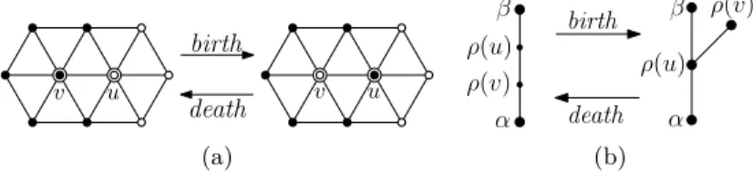
Maintaining Reeb Graphs of Triangulated 2-Manifolds ∗†
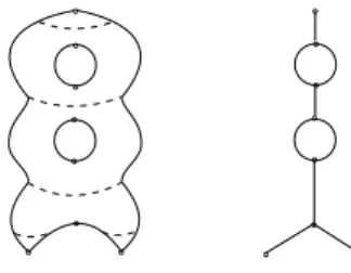
3 Time varying Reeb graph
4 KDS for R
Useful operations
5 Handling events
On the Parameterized Complexity of Simultaneous Deletion Problems ∗
3 From Simultaneous FVS/OCT to Colorful OCT
4 An FPT algorithm for finding colorful separators
Setting up the algorithm
5 W[1]-hardness of Simultaneous OCT
Swagato Sanyal 8
Anshu et al. 10:3
Anshu et al. 10:5
3 Composition Theorem
Anshu et al. 10:9
Anshu et al. 10:11
Verification of Asynchronous Programs with Nested Locks
3 Model
4 Undecidability of the Reachability Problem for Well-Nested N -MPDSs
5 Well-Nested N -MPDS under the Task Locking Policy
Serialized Executions
From N -MPDS to 1-MPDS
6 Stateless Well-Nested N -MPDS under the Task Locking Policy
Bartosz Bednarczyk 1 and Witold Charatonik 2
Bednarczyk and W. Charatonik 12:3
3 Finite words
4 Finite trees
5 Conclusions and future work
Bednarczyk and W. Charatonik 12:15
Béatrice Bérard 1 , Serge Haddad † 2 , and Engel Lefaucheux 3
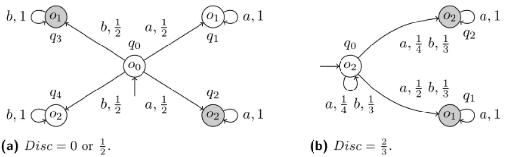
2 Specification
Opacity for Markov chains
Opacity for Markov Decision Processes
3 Maximisation with finite horizon
4 Minimisation with finite horizon
5 Fixed horizon problems 5.1 Maximal disclosure
Minimal disclosure
Olaf Beyersdorff 1 , Luke Hinde 2 , and Ján Pich 3
3 Strategy extraction and reasons for hardness
4 Hardness due to quantifier alternation
5 An alternative definition of hardness from alternation
6 Alternation Hardness of Specific Formulas
7 Conclusion
Amey Bhangale 1 , Subhash Khot 2 , and Devanathan Thiruvenkatachari 3
Previous Work
Proof Overview
2 Organization
3 Preliminaries
Analysis of Boolean Function over Probability Spaces
4 Query efficient Dictatorship Test
5 Analysis of the Dictatorship Test
Soundness
A Proofs of Lemma 11, 12 & 13
B Proof of Observation 8
Michael Blondin † 1 , Alain Finkel 2 , and Jean Goubault-Larrecq 2