9th Innovations in Theoretical Computer Science

Kousha Etessami, University of Edinburgh Oded Goldreich, Weizmann Institute Anupam Gupta, Carnegie Mellon University Zhiyi Huang, University of Hong Kong. Greg Valiant, Stanford University John Watrous, University of Waterloo David Woodruff, Carnegie Mellon University Yuan Zhou, Indiana University.

Barriers for Rank Methods in Arithmetic Complexity ∗†

Klim Efremenko 1 , Ankit Garg 2 , Rafael Oliveira 3 , and Avi Wigderson 4

To see how these barrier results directly affect the state of computational complexity, we note the following. Second, the above limits are far (quadratically removed) from the actual complexity (e.g. of random polynomials) in these models, which, if reached (by any means), are known to imply lower limits of the superpolynomial formula.

1 Introduction

• Sub-Additive Measures, Rank Bounds and Barriers
• Main results
• High-level ideas of the proof
• Related Work
• Organization

Abstracting all these examples and even most of the known lower bounds of arithmetic complexity5 can be done in a simple way. In both cases, our barrier results are close (to a function of d, the degree8) to the best explicit lower bounds (obtained by ranking methods), and are roughly squared away from the (desired) lower bounds that hold for arbitrary polynomials.

2 Rank Bounds

In another work, Razborov [44] showed how ranking methods can be used to prove superpolynomial lower bounds of monotone Boolean formulas. Then no ranking method using this linear map can prove lower bounds better than .

3 Conclusion and Open Problems

This is related to the minimum degree, combined with Corollary 14 and the fact that fi(x) andgi(x) are set-multilinear, gives. In Proceedings of the Thirty-seventh Annual ACM Symposium on Theory of Computing, pages 366–375.

A Preliminaries

General Facts and Notations

The degree of a polynomial f(x) ∈ F[x] with respect to a variable xi, denoted by degi(f(x)) is the maximum degree exi on a nonzero monomial off(x). The following lemma tells us that every nonzero polynomial cannot vanish in a large part of any sufficiently large network.

Matrix Spaces

The symbolic rank is important because it indicates the rank of the linear space of matrices, as can be seen from the following proposition. The following proposition shows one way in which a linear space is a low-rank matrix.

Coefficient Spaces and Their Properties

That is, the rank of the setMis given by the maximum rank (overF) among its elements. If f(x),g(x)∈ F[x]m are vectors of homogeneous set-multilinear polynomials, where(x) is partitioned with respect to the variables(xi)i∈Sf eng(x) is partitioned with respect up to the variables(xi)i∈Sg, then we have:.

B Restricted Forms of Symbolic Matrix Rank Decompositions

J Using this concept of mass-multilinear decomposition and the above lemma, we obtain the following relation between the symbolic rank and the mass-multilinear rank of a mass-multilinear polynomial matrix.

Asymmetric Spin Systems Using Number Theory

Jin-Yi Cai 1 , Zhiguo Fu 2 , Kurt Girstmair 3 , and Michael Kowalczyk 4

If the ratio of the two eigenvalues ​​is a unit root, an iteration of the construction will end up repeating after a fixed number of steps (up to a scalar). Unfortunately, it is actually possible for the ratio of eigenvalues ​​for one of the two constructs to be a root of unity, depending on the specificf.

2 A Theorem in Number Theory

There exists an odd Dirichlet sign χ (for n > 2): The group of Dirichlet signs mod n is isomorphic to Z×n. So we can define an odd Dirichlet signχ onZ×n by Chinese remaining by defining it to be odd on each Z×pei.

3 Definitions and Known Results

Gadget Construction

If f is realizable from the set F, then we can arbitrarily add f to F, preserving complexity. An F-gate (G, π) is similar to the signature network for Holant(F), except that G= (V, E, D) is a graph with some hanging D edges.

Tractable Signature Sets

Matchgates were introduced by Valiant [27] to provide polynomial-time algorithms of the FKT algorithm for a collection of counting problems over planar graphs. If z =w, y =x, where = ±1, then (=k |f) is M-transformable using the holographic transformation H by Lemma 7, and Pl-Holant(=k |f) can be computed in polynomial time with FKT algorithm.

Some results

We stratify the assignments in Ωl with nonzero scores based on the assignments to signature occurrences with the signature matrix h. We stratify the assignments in Ωl with non-zero scores based on the assignments of t occurrences of the signature with the signature matrix [10 1lλ].

4 Trichotomy for Spin Systems on 4-regular Graphs

This ratio is a root of unity if the complex argument ψ of a+ 2bi =|a+ 2bi|eiψ is a rational multiple of π, where cot(ψ) = 2ab. For the proof of these cases we finally use Theorem 1 from number theory. has infinite projective order, that is, the ratio of the eigenvalues ​​1+1−yiyi is not a root of unity.

5 Trichotomy for k-regular Graphs

ACM 60(5): 32:1-32:36 (2013)

10 Jin-Yi Cai, Michael Kowalczyk: Rotating regular-onk graph systems with complex edge functions. 11 Jin-Yi Cai, Michael Kowalczyk, Tyson Williams: Gadgets and anti-gadgets leading to a complexity dichotomy.

Quantum Query Algorithms are Completely Bounded Forms

Srinivasan Arunachalam ∗ 1 , Jop Briët † 2 , and Carlos Palazuelos ‡ 3

• The polynomial method
• Our results
• Related work
• Organization

The polynomial method is based on a connection between quantum query algorithms and polynomials discovered by Beals et al. 18] use the polynomial method to solve the quantum query complexity of several other well-studied Boolean functions.

2 Preliminaries

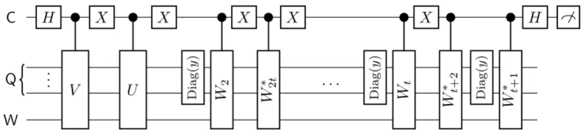
In all these settings, quantum algorithms constructed from polynomials were non-adaptive algorithms, i.e., the quantum algorithm starts with a quantum state, iteratively applies the oracle a fixed number of times, and then performs a projective measurement. Note that in this model, we are not concerned with the amount of time (i.e., the number of gates) it takes to implement the interpolation units, which can be much larger than the complexity of the query itself.

3 Characterization of quantum query algorithms

Let {P0, P1} be the two-outcome measurement performed at the end of the algorithm and assume that it returns +1 on measurement outcome zero and -1 otherwise. Note that we could also run the quantum algorithm forx /∈And let β(x) be the expected value of the quantum algorithm for suchxs.

4 Separations for quartic polynomials

Moreover, if we set Tσ=T for eachσ∈St, then from the above decomposition of Tpand definition 2 it follows that kpkcb≤ kTkcb≤1. From the union bounded over x∈ {−1,1}n it follows that kpk>2n2 with a probability of at most 2e−n, which yields the claim.

5 Short proof of Theorem 1

Now it is clear that the expected value of the measurement result is exactly (x)/KG, which gives Theorem 1 with C= 1/KG. Scope programs and quantum query complexity: The general adversarial bound is almost strict for every Boolean function.

A Complete Characterization of Unitary Quantum Space ∗†‡

Bill Fefferman 1 and Cedric Yen-Yu Lin 2

Background and Motivation

Recently, Ta-Shma [30], building on work by Harrow, Hassidim and Lloyd [18], showed that a well-conditioned×n matrix can be inverted (up to 1/poly(n) error) by a quantum O( logn ) space algorithm using intermediate measurements. Our completeness result for matrix inversion, together with the observation that our algorithm for matrix inversion (Theorem 14) actually gives a high-precision approximation, gives the following corollary in the logspace case (see Remark 2.3).

Relationship with Matchgates

In particular, our proofs use space-efficient methods for strengthening unitary quantum computations that are not known in the non-unitary model. By suitably bounding the dimension of the matrix and either the condition number or the lifting gap, we can render problems complete for quantum time or quantum space.

Quantum Merlin-Arthur with Small Gap

We know that sampling output distributions of passport calculations gives us the power of BPL; but what is the computing power to calculate exactly the output probabilities of matchgate calculations. It is known that output probabilities of passport calculations can be precisely calculated by an efficient classical algorithm [21], which is consistent with our conjecture because DET∈P.

2 Preliminaries 2.1 Quantum circuits

Space-bounded computation

This allows us to prove that testing whether a local Hamiltonian is frustration-free is a complete PSPACE problem (Appendix D). Our results show that if the promise gap is removed, then we obtain PSPACE completeness.

Other definitions and results

3 The Well-Conditioned Matrix Inversion Problem

We first briefly summarize the algorithm of Ta-Shma [30], which is based on the linear system solver of Harrow, Hassidim and Lloyd [18]. From here, our algorithm differs from Ta-Shma's and uses a combination of amplitude amplification and phase estimation.

4 The Minimum Eigenvalue Problem

We only provide a high-level overview of the proof here; for the full proof, see Appendix B. Again, we only give an overview; see the full version of the paper for the full proof.

5 Complete problems for time- and space-bounded classes

Combined with the perfect completeness results of Appendix C, this will also provide a proof that determining whether a local Hamiltonian is frustration-free is a PSPACE-complete problem (Theorem 35 in Appendix D). Given as input is the size-inefficient encoding of a2O(k)×2O(k)positive semidefinite matrix H with a known upper boundκ= poly(T) on the condition number, such thatκ−1IH I, and s, t∈ { 0 ,1}k(n).

6 Open Problems

These results interpolate between the time-bound and space-bound case: when T = poly(k) the time-bound case dominates and we obtain a time-bound class; while when T = 2O(k) we obtain a space bound class. In Proceedings of the 54th IEEE Annual Symposium on Foundations of Computer Science (FOCS), pages.

A More details on space-bounded computation

B Proof of Lemma 20

In-place gap amplification of QMA protocols with phase estimation

Removing the witness of an amplified QMA protocol

C Achieving Perfect Completeness for PreciseQMA

Since PSPACE=PreciseQMA, this proposition shows that any PreciseQMA protocol can be reduced to another PreciseQMA protocol with perfect completeness, i.e. U can therefore be implemented exactly in any gate set that allows Hadamard gates and Toffoli gates to be implemented exactly.

D Precise Local Hamiltonian Problem

E In-place gap amplification

Thus, the above procedure, which uses phase estimation applications to O(c−s) precision, can be implemented with a circuit of size O(rt/(c−s)) using O(rlog[1/(c−s)]) additional ancilla cubits. Using the standard in-place QMA error minimization analysis [ 24 , 25 ], it can be seen that this procedure has a probability of completeness at .

In the YES case, the measurement outputs 1 with probability at least c, whereas in the NO case, the measurement produces at most 1 with probability, with c > s. The standard counting argument that places BQPinside PP then also applies to this case; see e.g. [1, propositions 2 and 3].

Matrix Completion and Related Problems via Strong Duality ∗†

Our Results

Moreover, there exists a convex matrix completion optimization of the form (2) which exactly recovers X∗ with high probability, provided that m=O(κ2µ(n1+n2)rlog(n1+n2) log2κ(n1+n2 ) ), where κ is the number of conditions of X∗. There is a convex optimization formulation for robust PCA in the form of problem (2) which accurately recovers the incoherent matrix X∗∈Rn1×n2 and S∗∈Rn1×n2 with high probability, also cherrank(X∗) = Θ min{n .

Our Techniques

Thus, the finger shows the exact recoverability of inverse linear problems such as matrix completion and robust PCA, it suffices to study either the primal non-convex problem (1) or its convex counterpart (2). Our nonconvex geometric analysis is in stark contrast to previous convex geometric analysis techniques [56] where convex combinations of nonconvex constraints are used to define the Minkowski function (e.g., in the definition of the atomic norm) while our method uses itself the non-convex constraint.

3 ` 2 -Regularized Matrix Factorizations: A New Analytical Framework

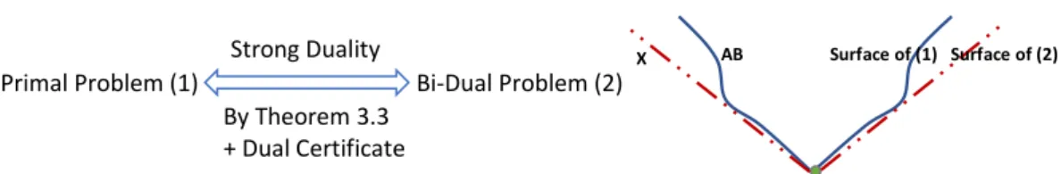
Strong Duality

If there exists a dual certificateΛe satisfying condition 2 and the pair (A,e B)e is a local minimizer of L(A,B,Λ)e for the fixedΛ, then strong duality holds. In the following (see Section B), we will demonstrate applications that, with randomness, obey this dual condition with high probability.

4 Matrix Completion

To show the dual condition in Theorem 4, intuitively, we need to show that the angle θ between the subspace T and Ψ is small (see Figure 3) for a specific function H(·). We show that the dual condition in Theorem 4 holds with high probability by the following arguments.

5 Robust Principal Component Analysis

When the sample size |Ω| gets bigger and bigger, the angle θ gets smaller and smaller (eg when|Ω|=n1n2, the angle θ is zero if Ω =Rn1×n2).

6 Computational Aspects

Solving a low-rank factorization model for matrix completion using a nonlinear successive overrelaxation algorithm. Mathematical programming calculation. Completing low-rank matrices with corrupt samples from few coefficients general basis.IEEE Transactions on Information Theory.

A Proof of Theorem 5

B Proof of Theorem 7

Assume that Ω is sampled according to the Bernoulli model with success probability p= Θ(nm . 1n2) and the incoherence condition (3) holds. According to Theorem 15, the operator p(PTPΩPT)−1 can therefore be represented as a convergent Neumann series p(PTPΩPT)−1 = P.

C Matrix Completion by Information-Theoretic Upper Bound

D Proof of Theorem 9

To rule out random algorithms that run in time 2α(n1+n2) for a function α of n1, n2 for which α= o(1), note that we can define a new problem which is the same as the problem (P) except for H's input Description is filled with a string of 1s of length 2(α/2)(n1+n2). However, if a random algorithm can solve it in 2α(n1+n2) time, then it runs in poly(N) time.

A Quasi-Random Approach to Matrix Spectral Analysis ∗†

Michael Ben-Or 1 and Lior Eldar ‡ 2

1 Introduction 1.1 General

• Main Contribution
• Prior Art
• Overview of the Algorithm
• Filter(A, m, δ )
• Compute parameters
• Sample random unit vector
• Approximate matrix exponent
• Raise to power
• Generate matrix polynomial
• Filter

A natural yardstick by which to test the novelty of the proposed algorithm is the iterative power method of computing the eigenvalues ​​of a Hermitian matrix. This allows a natural parallelization of the algorithm to extract simultaneous approximation of all eigenvectors.

2 Preliminaries 2.1 Notation

Definitions .1 Complexity

• Stable Computation

Letω denote the infimum over all such that any two n×n matrices can be multiplied by at most a number of products, and timeO(log(n)). Let D denote the discretization of C into bits as follows: each infinite-precision arithmetic operation is followed by rounding to bits.

3 Additive Perturbation

In fact, our main reason for using perturbation is to induce a distribution of eigenvalues. 9] have shown that applying additional perturbations to any Hermitian matrix using a well-known Wigner ensemble, a set of random matrices that generalize the GUE, actually causes the eigenvalues ​​of the perturbed matrix to reach a minimal inverse polynomial separation.

4 Low-Discrepancy Sequences 4.1 Basic Introduction

• Some basic facts
• The Good Seed Problem
• Finding Reasonably-Good Seeds Locally
• Low-Discrepancy from Gaussian vectors

The proof of this theorem is somewhat technical and is in the full version of the article. Consider the discrepancy of the distribution of us-dimensional series formed by taking integer multiples of XM.

5 A Filtering Algorithm

Filter(A, m, δ)

• Supporting Claims

Subsequently, driving ˜U to a power repeatedly takes a maximum of time: O(nωdlog(m)e) and driving B repeatedly to a power takes a maximum of time: O(nωdlog(p)e) So the total complexity is: O (nω log(pm/δ2)). So when we multiply two matrices at any of the steps above, both have at most 1 norm.

6 Sampling Separating Integers

Additive Perturbation

Approximate Pairwise Independence

Proof of Theorem 34

7 Parallel Algorithm for ASD

Initialize

Generate database

Non-Negative Sparse Regression and Column Subset Selection with L 1 Error

Aditya Bhaskara ∗ 1 and Silvio Lattanzi 2

Bhaskara and S. Lattanzi 7:3

• Our results
• Interpreting error bounds and comparisons to prior work

This method can be used to achieve a trade-off between the approximation of the objective and the sparsity of the solution obtained. The anchor word assumption states that X can be chosen to be a subset of the columns of M, reducing the problem to non-negative CSS.

Bhaskara and S. Lattanzi 7:5

2 Sparse recovery under noise

Analyzing the potential drop

As shown in the previous subsection, the key is to analyze the potential drop. In other words, we need to prove that there exists au∈V such that the above difference is "large".

Bhaskara and S. Lattanzi 7:7

J We are now ready to complete the proof of the main lemma of this section – Lemma 5.

Bhaskara and S. Lattanzi 7:9

3 Low rank approximation

Oracle for each iteration

Since this was also the challenge of Section 2, we begin by recalling a key aspect of the analysis: the definition of the truncated vectors w. Note that as everything is of the form Aj⊗z, we need to find az∈∆m that maximizes the objective value.

Bhaskara and S. Lattanzi 7:11

4 Solving the linear program efficiently

5 Conclusion

Bhaskara and S. Lattanzi 7:13

In Doina Precup and Yee Whye Teh, editors, Proceedings of the 34th International Conference on Machine Learning, ICML 2017, Sydney, NSW, Australia, 6-11. August 2017, volume 70 of Proceedings of Machine Learning Research, pages 806-814. In Peter Grünwald, Elad Hazan and Satyen Kale, editors, Proceedings of The 28th Conference on Learning Theory, COLT 2015, Paris, France, July Volume 40 of JMLR Workshop and Conference Proceedings, pages 696-709.

Bhaskara and S. Lattanzi 7:15

A Experiments

Spectrum Approximation Beyond Fast Matrix Multiplication: Algorithms and Hardness ∗

• Our Contributions .1 Upper Bounds
• Lower Bounds
• Related Work on Spectral Sums
• Algorithmic Approach
• Spectral Sums via Trace Estimation
• Singular Value Deflation for Improved Conditioning
• Further Improvements with Stochastic Gradient Descent
• From Linear System Solvers to Histogram Approximation
• From Histogram Approximation to Spectral Sums
• Lower Bound Approach
• From Schatten 3-norm to Triangle Detection
• Generalizing to Other Spectral Sums
• Paper Outline

Specifically, it is possible to approximately apply (ATA)−1 to a vector with the number of iterations depending on the average condition number: ¯κ=. Thus, an accurate approximation to this spectral sum allows us to determine the number of triangles inG.

3 Approximate Spectral Windows via Ridge Regression

Step Function Approximation

Ridge Regression

There is an algorithm that builds a preconditioner forMλ using O(nnz(A)k˜ +dkω−1) precomputation time for sparseAor O(nd˜ ω(logdk)−1)time for denseA, and for each input∈Rd, kthenx such that with high probability. There is an algorithm that builds a preconditioner for Mλ using precomputation timeO(nnz(A)k+dk˜ ω−1), and for each input y ∈ Rd, returns x such that with high probability.

Overall Runtimes For Spectral Windows

Due to the dependence on the mean condition number, the method always outperforms traditional iterative methods, such as conjugate gradient, up to log factors. Since a < b, the running time is dominated by the calculation of sγa(ATA)y, which depends on the condition number ¯κdef= kσ.

4 Approximating Spectral Sums via Spectral Windows

Approximate Spectral Histogram

In our final algorithms, the number of windows and samples required for trace estimation will be ˜O(poly(1/)). That is, ˜bbapproaches the number of singular values ​​of the rangeRtup to multiplicative (1±1) error and addition error dlog(1−α)λe ·2(bt−1+bt+1).

Application to General Spectral Sums

Application to Schatten-p Norms

Minimization of the number of arithmetic operations when solving systems of linear algebra equations. In Proceedings of the 51st Annual IEEE Foundations of Computing Symposium (FOCS), pp.

Size, Cost, and Capacity: A Semantic Technique for Hard Random QBFs ∗

Olaf Beyersdorff 1 , Joshua Blinkhorn 2 , and Luke Hinde 3

• Beyond propositional satisfiability
• When is a lower bound genuine?
• Random formulas
• Our contributions
• Organisation of the paper
• Quantified Boolean formulas
• QBF semantics
• QBF resolution

The present work embraces maximum generality and contributes a new technique for true QBF lower bounds in the general setting of P+∀red. The addition of universally quantified variables raises questions about which model should be used to generate such QBFs—care is needed to ensure an appropriate balance between universal and existential variables.3 The best-studied model is the model of ( 1,2)-QCNFs [22], for which bounds on the threshold number of clauses necessary for a false QBF were shown in [26].

3 Our framework

A formal definition of P+∀red

Before continuing, we extend our notation from PtoP+∀red the natural way, denoting the available lines in P+∀red (syntactically equivalent to the available lines in P) as LP+∀red, and write vars∃( L) and vars∀(L) for the subsets of vars(L), consisting of the variables that are existentially and universally quantized, with respect to the prefix of the input QBF. For formal definitions of the other propositional systems and their proof sizes, we refer the reader to the full article.

Propositional base systems

For each L ∈ LP and each partial assignment τ to vars(L), the Boolean functions BL[τ] and BL|τ are identical. The formalization of the framework of basis systems makes our technique applicable to the full spectrum of P+∀red-resistant systems.

4 Genuine QBF lower bounds with Size-Cost-Capacity

Defining cost

For any rowset L ⊆ LP and any rowL ∈ LP, L can be derived from LiffL semantically includesL;. All concrete propositional calculus considered in this work (i.e. those shown in Figure 1 ) are evidential basic systems.

Defining capacity

The Size-Cost-Capacity Theorem

For example, we prove that all QU-ResandCP+∀rerefutations have capacity equal to 1, and thus deduce that cost alone gives an absolute proof size lower bound there. Equipped with these results, which show that the cost of a QBF is superpolynomial, yields immediate proof size lower bounds for all three systems simultaneously.

5 Applications of Size-Cost-Capacity

The equality formulas: a new family of hard QBFs

The arguments for the QBF version of Polynomial Calculus with Resolution (PCR+∀red) are much more challenging and require some linear algebra, due to the underlying algebraic composition of Polynomial Calculus. Interestingly enough, it turns out that the capacity of a refutation there does not exceed its size, and thus the size of the proof is at least the square root of the cost.

The first hard random QBFs

The following theorem constitutes the first lower bounds on proof size for randomly generated formulas in the QBF proof complexity literature. We emphasize that these are true QBF lower bounds in the aforementioned sense; they are not just hard random CNFs lifted to QBF.

New proofs of known lower bounds

6 Discussion

Relation to previous work

The main drawback of the existing approach is of course the rarity of superpolynomial lower bounds of circuit complexity [55], especially for larger circuit classes to which the stronger QBF-proof systems connect. Instead, the lower bounds are determined directly from the semantic properties of the instance, and as a result we are advancing beyond the scope of previous techniques.

Innovations and future perspectives

A characterization of such lower bounds, and the proposal of associated lower bound techniques, would be an important development for the complexity of the QBF test.

7 Conclusions

In Fahiem Bacchus and Toby Walsh, editors, International Conference on Theory and Applications of Satisfiability Testing (SAT), volume 3569 of Lecture Notes in Computer Science, pages 502–518. Sakallah, editors, International Conference on Theory and Applications of Satisfiability Testing (SAT), volume 4501 of Lecture Notes in Computer Science, pages 355–368.

Paul Beame 1 , Noah Fleming 2 , Russell Impagliazzo 3 ,

Antonina Kolokolova 4 , Denis Pankratov 5 , Toniann Pitassi 6 , and Robert Robere 7

Beame et al. 10:3

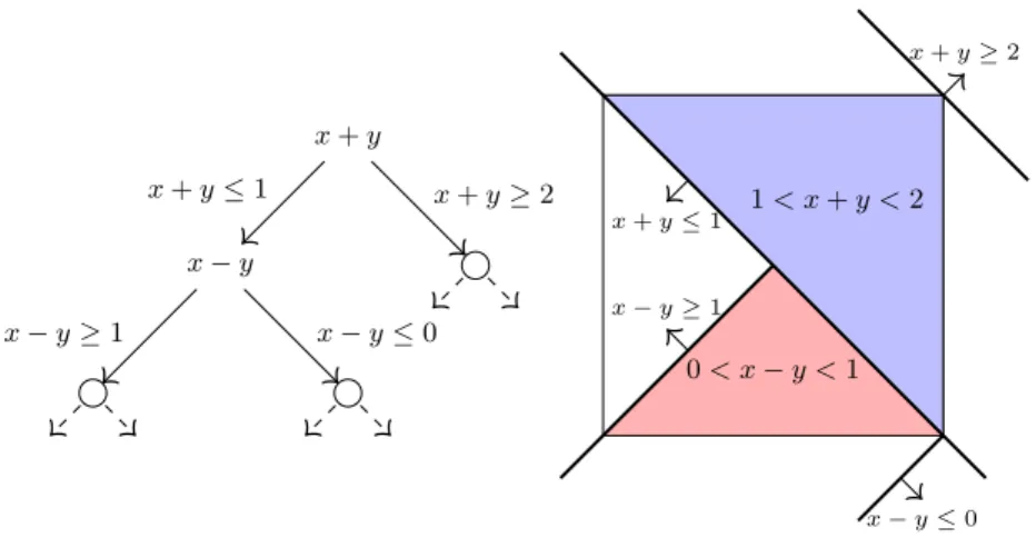
Each node of the tree after this substitution is now naturally connected to a polyhedral set Pu of points that satisfy each of the input inequalities and each of the inequalities on the path to this node. This opens up the space of algorithmic ideas considerably and should allow future pseudoBoolean solvers to take fuller advantage of the expressivity of linear integer constraints.

Beame et al. 10:5

This simulation provides new evidence of some depth lower limits that are already known in the literature; however, these lower bounds are supplemented by showing that neither SP refutations nor real communication protocols can be balanced. This should be seen in a positive light: the depth and size-complexity problems are really different for SP, and furthermore one cannot apparently obtain size lower bounds for SP by proving depth lower bounds for real communication protocols (as opposed to e.g. tree- like Cutting Planes).

Beame et al. 10:7