Combinatorial Pattern Matching

Maxime Crochemore King's College London, Great Britain and Universite Paris-est, France Travis Gagie University in Helsinki, Finland. Gregory Kucherov Universite Paris-Est Marne-la-Vallee, France Tak-Wah Lam University of Hong Kong, China.

Yoshifumi Sakai

1 Introduction

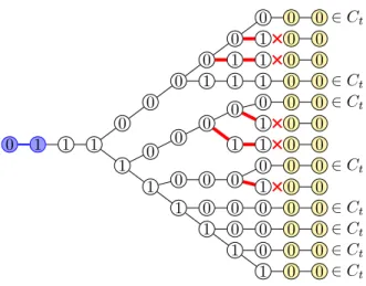
Possibly for an analogous reason, the best asymptotic running time known for finding a shortest maximal common sequence of two strings remains cubic [4]. This algorithm can also be used to find a bounded maximal common subsequence, thus having P as a subsequence, in the same asymptotic time and space, where P is an arbitrary common subsequence given as a "relevant" pattern .

2 Preliminaries

The present paper shows that, if we ignore such conditions regarding the length of a maximal common subsequence to be found, we can find a maximal common subsequence much faster in O(nlog logn) time, O( n) space algorithm. It is also shown that we can determine whether any given common subsequence, such as an RLCS, is maximal further faster by proposing an O(n) time algorithm.

3 Algorithm for finding a maximal common subsequence

Ifik+1becomestikorjk+1 becomesjk, and since (0, i0 ] (resp. Since C(W,W ,ˆ |W|) holds in the last execution of line 4 of the algorithm due to Lemma 4, it follows from Lemma 2 that the output of W by the algorithm has a maximum common is a subsequence of X and Y.

4 Algorithm for finding a constrained maximal common subsequence

Since lines 4 to 19 of the original algorithm do not delete characters from W, the modified algorithm eventually outputs the greatest common subsequence of X and Y containing P in O(nlog logn) time after initializing (W,W,ˆ 1) to (P, P,ˆ 1). Y(j,|Y|]) when executing line 9 of the algorithm are the shortest suffix X (or Y) containing P(k,|P|].

5 Algorithm for determining if a common subsequence is maximal

Each index in one (resp. the other) of the arrays in the pair is used to represent the last position at which a distinctive character in Σ appears in the prefix of Y (resp. The algorithm uses index variable ic (resp. jc) for each characterc in Σ. J) denotes the array consisting of variablesic (resp. jc) for all characterscin Σ.

6 Conclusion

For each sequence X and Y of length O(n) with|Σ|=O(n) and each common subsequence W of X and Y, Algorithm determineIfMCS outputs the message "not maximal" if W is not a maximal common subsequence of X and Y , or output the "max" message, otherwise, inO(n)time. The gap between the asymptotic running time of the proposed algorithms for finding a maximal common subsequence and for determining whether a given common subsequence is maximal immediately raises another natural question of whether we can find a maximal common subsequence in time O( n).

Indeterminate Strings

Rui Henriques

Alexandre P. Francisco

Hideo Bannai

Contrary to the great attention devoted to solving the OPPM problem, to our knowledge there are no polynomial-time algorithms for solving the µOPPM problem. Third, given a string of length, we show that the µOPPM problem is in polynomial time and linear space and is efficiently solved using efficient filtering procedures.

2 Background

The Problem

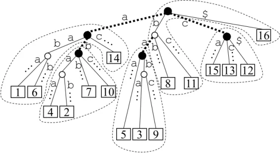
Given a totally ordered alphabet Σ, an indeterminate string is a sequence of disjunctive sets of charactersx[1]x[2].x[n] wherex[i]⊆Σ. Given an unspecified string x, a valid assignment $xis a (specified) string with a single character at position i, denoted $x[i], contained in the x[i] set of characters, i.e.

Related work

Given a given string x of length m, an indefinite string y of equal length is said to maintain order with respect to x and $y are the same, i.e. given a certain stringp of length and an indefinite string of lengths, the previous approach is a direct candidate for the µOPPM problem by decomposing O(rn) into all its possible assignments.

3 Polynomial time µOPPM for equal length pattern and text

O(mr lg r) time µOPPM when one string is indeterminate

By ordering the characters in descending order per position, we guarantee that at most one character per position in y0π appears in the LIS (respecting the monotonic ordering inxgiveny0πproperties). Given the fact that the candidate string for the LIS task has properties of interest, we can improve the complexity of this calculation (Theorem 2) in accordance with Algorithm 1.

O(m 2 ) time µOPPM (r=2) with indeterminate pattern and text

J If the establishedφformula is satisfiable, there is a Boolean assignment to the variables that specifies an assignment of characters iny, $y, preserving the orders ofx (as defined by Leq,Lmax andLmin). J If the formula is satisfiable, there is a Boolean assignment to the variables so that there is an assignment of characters in y, $y, and in x, $x, so that both strings match.

4 Polynomial time µOPPM

Given Theorem 11 and the ability to solve 2SAT problems linearly in the size of the CNF formula [10], the proof of this theorem follows naturally. Instead, the complexity of the proposed method for solving the μOPPM problem becomes O(dmrlgr+n) (when one array is undefined) or O(dm2+n) (when both arrays are undefined dher=2) where number of correct matches ( dn ).

5 Concluding remark

The properties of the proposed encoding guarantee that the exact matches of p0 in t0 cannot skip any up-match ofpint. On tuning the (δ,α)-sequential sampling algorithm for δ-approximate matching with alpha-bounded gaps in musical sequences.

Burrows-Wheeler Transform

Uwe Baier

This was reasonable because, also stated by Fenwick [6], "the original scheme proposed by Wheeler is extremely efficient and is unlikely to be much improved." Finally, the global skewed character distribution of the transform is useful for the final stage of typical BWT compressors: entropy coding.

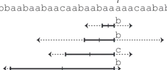
3 Tunneling

Another trick for improving compression used by most advanced BWT compressors is run-length encoding. We would also like to note that each column of a block can be mapped to a substring in the BWT that consists of the same character.

4 Invertibility

As a remainder, tunneling means we remove all the characters except the rightmost and leftmost columns and the top row of a block. In blocks, we know that every row in the block is identical, and all the rows run in parallel (in terms of LF mapping).

5 Practical Implementation

Block Computation

Each time a run is reached that allows the current block to be expanded in width, the current block is pushed onto a stack and the run is used as a new block. Once the current block cannot be expanded (because the current run is not high enough), blocks are removed from the stack until an expandable block is reached.

Tunneled BWT Encoding

Data: a set of width-maximal run blocks and a function count that returns for each block the amount of run characters it removes. Since most modern compressors use run-length encoding, we estimate net benefit and tax in terms of run-length encoding.

Block Choice

Count updates of outer collisions are approximated by multiplying the count by the ratio by which the block width is shortened. If the middle block has a score greater than that of the outer blocks (but close enough), fort= 1, the middle block is the optimal choice, while for t = 2 the outer blocks will be preferred, which is not by the algorithm.

6 Experimental Results

Boxes consist of lower quantile, median, upper quartile and mean (red dashed line), whiskers are indicated by 1.5 times the interquartile range, outliers are shown as diamond markers. Compression improvements use the non-tunneled versions as baseline, model fits are given by the min-max distance of the gross-net benefits ratio for theoretical model and compressor.

7 Conclusion

It would also be nice to get rid of the limitation of run-based blocks; Section 5.1 indicates that this is possible, but collisions complicate the situation. Thinking of a text index with half the size of the currently best implementations seems utopian, but this paper shows that this goal should be achievable, giving much motivation for further research on the topic.

Amihood Amir

Avivit Levy

Ely Porat

Properties of Covers and Seeds

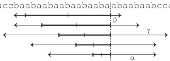
If nizc is a cover of W, then the seed of every factor of W is of length at least |c|. However, if we take W2=ababaababaa, which is still periodic with p, but can no longer be covered by ciabe (which remains its seed).

3 Quasi-Periodicity Persistence Under Mismatch Errors

Note that by Lemma 15 any quasi-periodic string with only two occurrences of the cover is periodic, for which Observation 22 applies. So inAC we have two consecutive occurrences of ˆc, where ci is a suffix of the first occurrence (due to the occurrence of ofc in indexes+|c0| − |c|) and a prefix of the second occurrence (due to the fact that this is a prefix is of ˆc), and there is overlap between the suffix of the first and the prefix of the second (due to its occurrence in in indexr).

4 Application: Closing the Complexity Gap in ACP Relaxations Study

The Histogram Greedy Algorithm

Find m, the length of an estimated cover subject to the tile L, by calculating the difference between n+ 1, and the last index in the tile L, Llast, which indicates the last occurrence of the cover inT. As discussed in [5], the output C of the Histogram Greedy algorithm may not be an L-approximate coverage of T because it may not be primitive, as the following example shows.

The Full-Tiling Primitivity Coercion Algorithm

To impose the requirement that the definition of an L-approximate covering of T must be a primitive string such that all its repetitions for covering (with minimum number of errors) are marked in the tiling L, we need a primitiveness constraint algorithm. The following subsection is devoted to proving the correctness of the full-tiling primitiveness constraint algorithm, thus proving that the full-tiling relaxation of the ACP is polynomial-time computable.

Correctness of the Full-Tiling Primitivity Coercion Algorithm

Then assume that C0 is not a primitive string and therefore the second step of the Full-Tiling Primitivity Coercion algorithm is performed. The second step of the Primitivity Coercion algorithm for full tiles selects a character that minimizes the difference H(SL(C0), T)−H(SL(C), T.

Maximum Duo-Preservation String Mapping and its Weighted Variant

• Problem Description
• Related Work
• Our Contributions
• Preliminaries

We show a transformation of the Maximum Duo-Preservation String Mapping (MPSM) problem into a related solvable problem. A correct mappingπfromAto B is a one-to-one mapping from the letters ofAto the letters ofB withai=bπ(i) for alli= 1,.

2 Main techniques and algorithm for MWPSM

The Alternating Triplet Matching (ATM) problem

A pair of pairs (DAi , DBj) is called conserved if and only if fai=bj anddai+1=bj+1. In the case of multiple edges between a pair of triplets (e.g. five edges between "AAA" triplets), we show only the heaviest edge.

MWPSM algorithm and analysis

Thus, we can only keep the weight of one of the two pairs in our ATM solution. We can now show how to convert the optimal ATM solution (the more difficult of the two matches) into a feasible string mapping that preserves at least half the weight of the ATM solution.

3 Linear time algorithm for unweighted MPSM

First, we note that each duo contains at most one triple edge from the ATM solution and therefore can only be matched once in M. We can also show that at most one type 2 conflict arises at each endpoint .

Solving b-ATM quickly

As in Section 2.1, let OP TG0 and OP TG00 be the weights of maximum weight b-matches in G0 and G00, respectively. Given a maximum weight b-matchingM that does not include all identical pair edges, we can always add one such edge without reducing the weight of the solution.

Transforming the b-ATM solution to a duo matching and resolving conflicts

1 Assign each copy of a 3-more and its edge of the b-ATM solution to a triplet of the original strings to get an ATM solution. Since he has a weight of 2 while the removed edges have weights of 1 each, swapping those edges will not reduce the weight of the solution.

4 A streaming algorithm for MPSM

5 Conclusion and future directions

The complementary relationship with Minimum Common String Partition (MCSP) has fueled much of the current interest in MPSM. InProceedings of the 15th International Conference on Algorithms and Computation, ISAAC'04, pages 484-495, Berlin, Heidelberg, 2004.

Guillaume Blin

Élise Vandomme

Words

Taking a word∈Σ∗, we say that it is a factor iw∈Σ∗ if there are two wordsx, z∈Σ∗ such that w=xyz. Two wordswandw0 are conjugate, denoted mew∼w0, if there exist two wordsxand y such that w= xy andw0 = yx.

Problem definition

In the following, each runy is considered maximal, that is, the last letter ofx and the first letter ofz are both different from a. For one such example, let ugreedy&circ∈C1 be the word obtained by concatenating the last two runs of ugreedy into a run of 0 or 1 (whichever gives the smallest distance draw).

3 Computing the optimal distance for a fixed irradiation time

Distance matrix

To calculate the quantity Solt(w), we build a dynamic matrix using the possible prefixes for u∈Solt(w), i.e. the quantity. Note that the size of the matrix Dw,t,p, which is equal to |At∩ {0, t}`| ×n, is polynomial with respect to `andn.

Dynamic programming

The extensions highlighted in red are therefore not prefixes of any circularly admissible words and should therefore be discarded. Therefore, for n−cp < i ≤n, every u∈ Ct,p(v, i) is a prefix of a circularly admissible word and must end with pi−n+c1 p.

4 Computing an optimal solution

An arrow between two cells indicates that the value in the arriving cell is calculated from the one in the originating cell. In bold is a path corresponding to an optimal solution (not necessarily unique) for the irradiation time 2.

5 Forbidding overdoses

Letv be the jth conjugate of andw0 be the jth conjugate of w, for an integer such that1≤j≤n. Since v is the jth conjugate of u and w0 is the jth conjugate of w we have thatv=uj.

6 Perspectives

Although the complexity in the worst case is not improved, in many cases the number of distance matrices to be calculated is significantly reduced. For example, the following example shows that instead of the 30 distance matrices needed to find the optimal solution in the original setting, only one distance matrix is ​​needed for the "no overshoot" problem.

RLBWTs

Policriti and Prezza’s augmented RLBWT

The result of Policriti and Prezza can be somewhat simplified and strengthened by storing only the position of the first character of each run and finding the initial position of the lexicographically first suffix that begins with the given pattern. When we start looking back for the pattern P[1.m], the starting interval is all of BWT[1.n] and we know SA[1], since BWT[1] must be the first character in the string.

Updating an RLBWT

Otherwise, the range for P[i−1.m] starts with BWT[LF(j0)], where j0 is the position of the first occurrence of P[i−1] in BWT[j.k]; since BWT[j0] is the first character in a run, j0 is easy to calculate and we have SA[j0] saved and can thus calculate SA[LF(j0)]. We can augment an RLBWT with O(r) words in which the number of runs in the BWT such that after each step of a backward search for a pattern we can return the starting position of the lexicographically first suffix preceded by the suffix of the pattern we have so far processed.

3 Online LZ77 Parsing

Updating an augmented RLBWT

We replace $ byT[i] in RLBWT, which may require that copy of T[i] to be merged with the previous run, the subsequent run, or both. We can build an RLBWT for TR incrementally, starting with the empty string and iteratively preceding T[1],.

Computing the parse

Experimental results

For the non-rle-lz77-2 methods above, the output space is not counted in the workspace because they compute the LZ77 phrases sequentially. We can see that the rle-lz77-ogets workspace is worse as the input is less compressible compared to RLBWT (especially for Escherichia_Coli).

4 Matching Statistics

Further augmentation

By definition of BWT, the length of the longest prefix in common with the suffix eT starting from the copy of c before BWT[i], is not increasing as we move from BWT[i] to BWT[k], and the length of the longest prefix common length with suffix eT starting from copy ofc after BWT[k] is not descending; therefore there exists at most one such threshold j. Handling special cases, such as when evencT[SA[i].n] has a longer prefix in common with the suffix eT starting from the copy ofc after BWT[k], takes a constant number of bits addition, so in total we use O(rσ) space for this addition, where is now the number of runs in BWT forT (not TR).

Algorithm

Application: Rare-disease detection

For simplicity, we ignore special cases, such as when a certain character inS does not appear inT. Again, for simplicity we ignore special cases, such as when a certain character in S does not appear in T.

5 Recent and Future Work

Në Proceedings of the 23rd Symposium on String Processing and Information Retrieval (SPIRE), faqet 1–14, 2016. Në Proceedings of the 22nd Symposium on String Processing and Information Re-trieval (SPIRE), faqe.

Sahar Hooshmand

Paniz Abedin

Oğuzhan Külekci

Thankachan

1 Introduction and Related Work

Popular computing models are (i) cache-aware model and (ii) cache-forget model. There is an O(nlogn) space data structure for the non-overlapping indexing problem in the forgotten cache model, where is the length of the input textT.

2 An Overview of Our Non-Overlapping Indexing Framework

Handling aperiodic case

For our problem, we use both the suffix tree and its cache-oblivious equivalent from Brodal and Fagerberg [4], which takes up O(n) space and can compute in optimal O(p/B+ logBn) I/Os. Let Q be the shortest prefix of P, so that P can be written as the concatenation of α ≥1 copies of Q and a (possibly empty) prefix R ofQ.

Handling periodic case

An instance is a cluster head (resp. cluster tail) if it is the first (resp. last) instance within a cluster. Let Ci be the i-th leftmost cluster and Si(resp., Si∗) the largest set of non-overlapping occurrences inCi including (resp., excluding) the first occurrenceL0[i] inCi.

3 Preliminaries for Missing Proofs 3.1 Heavy Path Decomposition

Right-Maximally-Periodic Prefixes

For a fixed suffixT[i, n], letl1, l2, .., lk be the length of all right-maximal-periodic prefixes in their ascending order and q1, q2, .., qk be their respective periods.

3.3 1-Sided Sorted Range Reporting

4 Proof of Theorem 2

5 Proof of Lemma 3

6 Proof of Lemma 7

Case 1: locus(P ) and locus(QP ) are on different heavy paths

In light of the above lemma, when the query P falls in this case, we can actually generate the final output directly instead of first generating L00 and using it. First obtain all occurrences of P in the sorted order (using the structure in Theorem 2) and extract the largest set of non-overlapping occurrences from them by following exactly the same procedure as in aperiodic cases.

Case 2: locus(P ) and locus(QP ) are on the same heavy path

• The Data Structure
• The Algorithm

Then retrieve the elements in the next two arrays in sorted order SA[·] via queries on the one-way sorted range reports.

7 Proof of Lemma 8

8 Concluding Remarks

Dehne, Jörg-Rüdiger Sack and Norbert Zeh, editors, Algorithms and Data Structures, 10th International Workshop, WADS 2007, Halifax, Canada, August Proceedings, volume 4619 of Lecture Notes in Computer Science, pages 625-636.

Kotaro Aoyama

Yuto Nakashima

Shunsuke Inenaga

Masayuki Takeda

A string matches an ED string if it is a substring of a string that can be obtained by taking a string from any position of the ED string and concatenating them. For space complexity, we will also assume that the strings at each position of the ED string are given in lexicographic order.

2 Preliminaries 2.1 Strings

Elastic-Degenerate Strings

An elastically degenerate string, or ED string, over alphabet Σ is a string over ˜Σ, that is, an ED string is an element of ˜Σ∗. Given a string P of length m, and an ED string T˜ of length and size N ≥m, output all positions j in T˜ where at least one occurrence of P ends.

3 Tools

Suffix Trees

For each node in the suffix tree, letstr(u) denotes the chaining of all edge labels to the root toupath and letlen(u) =|str(u)|. Given the suffix tree ST(w)for stringw, Occ(w, s) for any string can be computed in O(|s|+Occ(w, s))time.

Sum Set and FFT

Letparent(u) denotes the parent of u, andanc(u), desc(u), respectively, the set of nodes in the suffix tree that are ancestors and descendants of u, including itself. A position in the suffix tree can be represented by an a-pair (u, d), where u is a node and d≥0 is an integer such that d≤ |str(u)|ogd >|str(parent(u))|( ifparent( u ) exists).

4 Algorithm

• Overview of Algorithm
• Computing Step 1
• Computing Step 2
• Computing Step 3
• Computing S i =
• Computing S i <

This can be checked as follows: For each string t ∈T˜[i], traverse the suffix tree from the root witht. Since the sets can be computed in O(m) time, the sum set can be computed in O(mlogm) time using Lemma 4.

5 Conclusion

T˜[i][|T˜[i]|] are lexicographically ordered, we can reduce the space by doing the computation through a left-to-right depth-first traversal of the suffix tree, during which we keep only the locations on the route we are considering. If we cannot assume that the strings in each ˜T[i] are in lexicographic order, the space complexity becomes O(m+ maxi=1,..,n|T˜[i]|).

Tatsuya Akutsu

Colin de la Higuera

Takeyuki Tamura

In this paper, we focus on planar graphs, which is a planar graph with planar embedding, and present a (conceptually) simple linear-time algorithm to compute the canonical form of a planar graph. Of course, it seems possible to modify the algorithm in [11] for computing the canonical form of a planar graph while preserving the linear time complexity.

We assume that a face graph is given in a form of the double-linked-edge-list (DCEL) [17] so that the removal of an edge can be done in a constant time and the removal of a face can be done in time-proportional to the number of surrounding edges.

4 Linear time canonical form computation

If no single exposed face or edge exists in G, then Gi is a vertex, an edge, or a face (possibly including additional subgraphs within). The peeling process can be performed by removing edges in lists with individually visible flags.

5 Canonical form of geometric plane graphs

Since each edge is newly exposed only once and deleted only once, the total time complexity is proportional to the number of edges (ie, the total complexity is O(n)). Since the canonical form of a circular array over a general alphabet can be computed in O(n) time [6, 12], the total time complexity is O(n).

6 Maximum common connected edge subgraph of geometric plane graphs

Then the largest total connected edge subgraph can be computed in O(f(Df, Dv, K)n)time, where f(Df, Dv, K) =Df2·DvKDf2+Df+4. On the complexity of the maximum common subgraph problem for partial k-trees of limited degree.

Efficient Dynamic String Algorithms

Itai Boneh

The first problem we solve is the dynamic LCF problem for the decremental dynamic model. The second problem we solve is the FDOS-LCF problem in the special case where S is periodic.

3 Algorithm’s Idea

The Suffix Tree

Thus, each trie node in the suffix tree can be represented by the edge it belongs to and an index within the corresponding path. In standard suffix tree implementations, we assume that each node of the suffix tree can access its parent.

Preprocessing

Let us now examine the effects on the LMCFs of a substitution of ω for the symbol at index k of D. Clearly, all LMCFs ending before indexk and all those starting after indexk are unaffected.

4 Implementation 1: O(log n) Query Processing

We need a data structure that allows us to efficiently delete the corresponding LMCF arrays, add two new LMCFs if necessary, and efficiently find the largest one. The LMCF can be found in the suffix tree, as shown in subsection 3.2, in linear time.

5 Implementation 2: O(log log n) Query Processing

Data Structures

An interval tree is a fast tree sorted by the initial indices of valid intervals in the range {1, .., n}. A maximum-length tree is a fast tree whose entries are of maximum LMCF length in valid intervals.

The Algorithm

Similarly, updating the maximum length fast tree takes O(log logn) time, for a total of O(log logn) time. Find maximum length LMCF: Find the maximum element in the root maximum length fast tree.

6 Dynamic LCF for a Static Periodic String

Algorithm’s Idea

There are only O(p) "close" LMCFs, so they can be handled in a brute force manner and still cost only O(p) per query. The two lemmas guarantee a constant number of affected "far" LMCFs, so they are also handled efficiently.

7 The algorithm

Correctness

Another useful property of “far” LMCFs is that even if the edit operation truncates them - they are still at least of size p in the updated D . This can be done by locating the first instance of the new LMCF and using its knowns. size to find out if it is actually a factor.

Complexity

It finds the LCF of a dynamic string D and some infinite period of the first letters S. For simplicity, we presented the algorithm assuming a suitable length of S.

8 Conclusions

Any other size of S will bring into play the question mentioned in the note following the proof of the two lemmas in Subsection 6.1. If it isn't - then the starting index of its LMCF and its length can be used to derive the way it should be split in O(1) time.

Mitsuru Funakoshi

It was pointed out in [2] that Manacher's algorithm actually computes all maximal palindromes in the string. We also consider a more general variant of 1-ELSPal queries, where an existing substring in the input stringT can be replaced by a string of arbitrary length`, called an`-ELSPal query.

Related work

In the next section, we will present an O(n) time and space preprocessing scheme so that subsequent 1-ELSPal queries can be answered in O(log(min{σ,logn})) time. In the next section, we will propose an O(n) time and space preprocessing scheme so that subsequent `ELSPal queries can be answered in O(`+ logn) time.

3 Algorithm for 1-ELSPal

• Periodic structures of maximal palindromes
• Algorithm for substitutions
• Algorithm for deletions
• Algorithm for insertion
• Hashing

To calculate the length of LSPals from T0, it is sufficient to consider the largest palindromes from T0. It is possible to preprocess T in O(n) time and space, so that later in O(log(min{σ,logn})) time we can calculate the length of the longest largest palindromes in T0, which are.

4 Algorithm for `-ELSPal

We can calculate the length of the longest maximal palindromes whose centers are inside X inO(`) time and space. Therefore, it takes O(`) time to compute the length of the longest maximal palindromes whose centers are inside X.

Distance Computation and One-against-many Banded Alignment

Related Work

The Four Russians speedup, originally proposed for matrix multiplication, has been adapted to many problems beyond edit distance, including: RNA folding [10], transitive closure of graphs [20], and matrix inversion [4]. One-to-many edit distance comparison involves comparing a single string to a set of n other strings.

Preliminaries

• The classical Four Russians speedup

The block function takes as input the two substrings to be compared in that block and the first row and column of the block itself in the dynamic programming table. In practical applications of four-Russian acceleration, where space efficiency is important and smaller block sizes k are used (especially k < |Σ|), [13] showed how to remove the alphabet size dependence for the unit cost version, where created a lookup table in O(32k(2k)!k2) time and O(32k(2k)!k) space.

2 Storing and querying the block function

• Notation
• Storing lookup entries
• Querying a block function
• Alternatives to query a block function without SMAWK

Given the input row and column vectors and an O(k)×O(k) search input matrix M, we can compute the output row and column in O(k) time using the SMAWK algorithm [2]. First, we find the smallest value in row|V|/2 and let mincol be the column containing that cell.

3 One-against-many comparison

Extending the Four Russians approach to banded alignment

Looking ahead, we note that neither SMAWK nor the algorithm in this section utilizes all the specific properties of the matrixM0. Right: use these blocks to cover the diagonal band of the dynamic programming table in the context of band alignment.

Our algorithm

The time required to compute the block functions for difference comparisons between and all n other strings isO(nd3). Thus, the running time to compute the full dynamic programming for the difference blocks for all pairwise comparisons is O(n·d·d2) =O(nd3).

4 Extensions and applications

Comparing two arbitrary strings with a penalty matrix

Excluding the time to compute the block functions for difference comparisons, the time to compare a string of length pof m with other strings using the precomputed lookup table isO(nm). If a block corresponds to an identity comparison that requires, the block function takes time O(k) =O(d) by Theorem 1.

Improved space-efficiency

Otherwise, if it's a difference comparison block, the only time will come from checking the lookup table, which we've assumed takes O(d) time. It follows that for a given pair of strings, the number of block queries corresponding to differences can be at most 2(d+ 1) =O(d), since we will stop a comparison if the distance ever reaches d+1 or more.

Exploiting prefix similarity in one-against-many comparison

In Russell Schwartz and Knut Reinert, editors, 17th International Workshop on Algorithms in Bioinformatics (WABI 2017), volume 88 of Leibniz International Proceedings in Informatics (LIPIcs), pages 3:1–3:13, Dagstuhl, Germany, 2017. A space -efficient alphabet - independent lookup table of four Russians and a multithreaded edit distance algorithm of four Russians.

Shu Zhang

Daming Zhu

Haitao Jiang

Jingjing Ma

Jiong Guo

Haodi Feng

Happy permutation

Formally, the pair consisting of πi and πj is an inversion of πi and πj into π, if i < j and πi> πj. For an element πi inπ, we refer to the entire interval [i, πi] as the vector i πi inπ and denote it asvπ(πi), where |vπ(πi)|=|πi−i| referred to as thelengthofvπ( πi).

Lucky permutation

An inversion inπ refers to a pair of elements that are not in their correct relative order. If π6=ι, there is at least 1 inversion of two adjacent elements inπ, which can be eliminated by a short swap.

3 How to recognize a happy permutation

We devote ourselves to showing that all unsorted MISPs in π0[x→y] must satisfy these two properties of Theorem-5. The rightmost vector right element inπ must be the rightmost vector right element in MISP inπ.

4 How to recognize a lucky permutation

A position-even (or position-odd) element iπ remains position-even (or position-odd) in π·ρhi, i+ 2i. Since π satisfies the theorem-19 property (1), an even (resp. odd) element inπ must be position-even (resp. position-odd).

Takafumi Inoue

Heikki Hyyrö

We show that the thek-LCSqS problem is at least as hard as the 2k-LCS problem, which asks to compute the LCS for 2kgiven strings. Our results for the LCSqS problem can be seen as a generalization of these results for the LSqS problem.

3 Algorithms

Simple Algorithm

In other words, a subsequence of Y can be obtained by removing zero or more characters from Y. The k-LCS problem is to compute the length of the longest common subsequence (LCS) given k strings where k≥2. Ak) denote the length of the longest common subsequence k of the sets A1,.

O(σ|M| 3 + n)-time algorithm

Thus, all sequences of DOMRs beginning with rectangles1 and ending with rectangles share the same unique dominant extensions. For each such starting rectangle rb, we compute a dynamic programming tableDPrb of size O(|M|2) such that DPrb[re] will eventually store the length of the longest sequence of DOMRs beginning withrb and ending withre, where is either rb itself or a dominant extension.