A workpiece for track B is accepted if and only if it is accepted by at least one of the two PCs. The Best Student Paper Award for Track A was awarded to Maximilian Probst for the paper “On the Complexity of the (Approximately) Nearest Colored Node Problem”.
Track A (Design and Analysis) Program Committee
Track B (Engineering and Applications) Program Committee
Arnold Filtser Anja Fischer Felix Fischer Matthias Fischer Till Fluschnik Dimitris Fotakis Kyle Fox Tom Friedetzky Tobias Friedrich Alan Frieze Zachary Friggstad Ulderico Fugacci Toshihiro Fujito Ben Fulcher Radoslav Fulek Travis Gagie Waldo Gálvez Guilhem Gamard Arun Ganesh Arnab Ganguly Wilfried Gan sterer Naveen Garg Bernd Gärtner Paweł Gawrychowski Rong Ge . Jean-Florent Raymond Ilya Razenshteyn Igor Razgon David Renault David Richerby Havana Rika Matteo Riondato Lars Rohwedder Clemens Rösner Günter Rote Eva Rotenberg Alan Roytman Paweł Rzążewski Yogish Sabharwal Kunihiko Sadakane Barna Saha.
Sara Ahmadian
Laura Sanità
1 Introduction
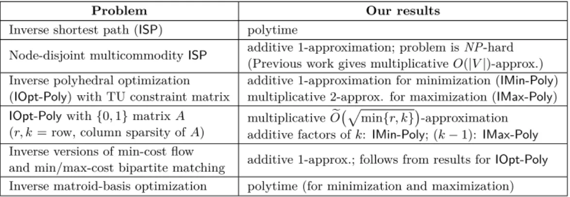
We obtain approximation guarantees for polyhedral inverse integral optimization that depend on the structure of the constraint matrix Definition P. In contrast, in setting inverse integral optimization, two distinct sources of difficulty arise that do not appear in the above setup.
2 Problem definitions, notation, and preliminaries
If the underlying discrete optimization problem is captured by an optimization problem over P (eg, if the extreme points of P correspond to feasible solutions of the discrete optimization problem), then this integral inverse polygon optimization problem captures the integral discrete optimization problem the inverse defined earlier. Inverse polyhedral integral optimization can be stated geometrically as: determine ifX forms a face, sayF, ofP, and if so, find a positive, integral (if any) minimal vector.
3 The inverse shortest path problem
A polynomial time exact algorithm for ISP
Furthermore, given the cost {bi}ni=1, we can solve a min-cost flow problem to find an optimal solution for the following LP: minimize P. We can efficiently solve (ISP-P) via the ellipsoid method , because we can efficiently solve divide over constraints (4) when c≥0 by solving a shortest path problem.
Multicommodity ISP with node-disjoint subgraphs
We can also use depth-first search and backtracking to enumerate |S|+ 1 distinct paths t in the polynomials (if they exist); see, e.g., [21].). We can assume that every edge∈E1 lies in ans the path contained in E1 (which lies by definition in the explicit model); otherwise, we can drop fromE1 and solve for the resulting instance ISP.
4 Inverse polyhedral optimization
Applications to inverse min-cost flow and inverse bipartite matching
In the integral inverse min-cost flow (IMCF) problem we get a directed graph D= (N, E), integers 0≤`e≤ue on each edge, integers require {bv}v∈N (which could be arbitrary ) so that b(N) :=P. In the implicit model we get E1⊆E, and the set of perfect matches with minimum cost should be the set of perfect matches in E1.
5 Inverse matroid-basis optimization
We also consider the bilateral integral min-cost matching (IMin-BMat), where we are given the perfect matchingsM1,. Mk, and we seek the positive integral costs of the edges{ce}e∈Eminimisingkck∞ such that these are the unique perfect min-cost matchings inG.
6 Extensions and variants
The min-cost perfect matching problem can be modeled by the following LP: min P. The constraint matrix in the above LPs is TU and has column sparsity 2. Non-approximability results for the inverse shortest path problem with integer lengths and unique shortest paths.
Shoshana Marcus
However, the notion of maximal two-dimensional iterations has not been investigated, either from a combinatorial or an algorithmic perspective. The discovery of repetitive structures in a two-dimensional sense can lead to improvements in compression schemes used for images and video.
2 Related Work
They develop an O(n3logn) algorithm for finding side-splitting tandems in an n×n matrix, which can be used to derive an O(n4) algorithm for finding all corner-splitting tandems [4] .4 In this paper we extend Apostolico and Brimkov's concept of a side-sharing 2D tandem to many copies to form maximal tandems horizontally and vertically. In this paper we discuss periodicity where partial copies are allowed at the ends of the matrix, i.e.
3 Definition of 2D Maximal Repetition 3.1 1D Maximal Repetitions
Apostolico and Brimkov [3], at the beginning of the above-mentioned paper on tandem, define exactly this kind of repetition. The rectangular lattice periodicity is also used by Gamard and Richomme [11] where the primitive roots of 2D arrays are studied.
3.2 2D Maximal Repetitions
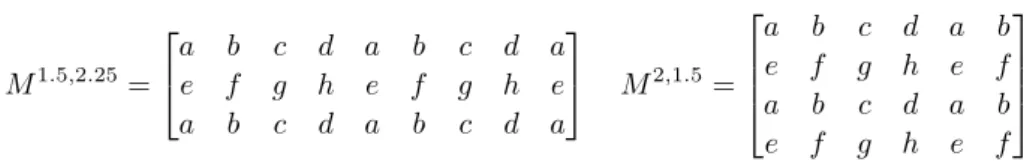
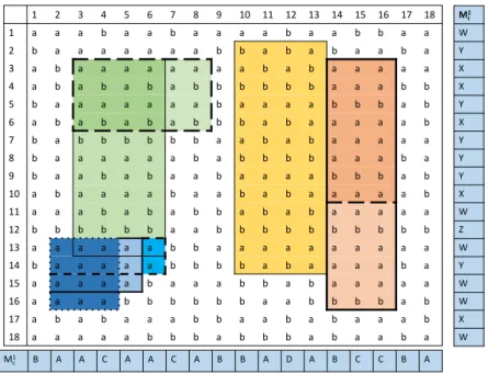
That is, the primitive root W is iterated both to the right and below its initial occurrence in R. A 2D iteration R with root W is maximal if it cannot be extended by one row or one column to obtain a 2D iteration with the same root W primitive.
4 Bounds on the Number of 2D Maximal Repetitions
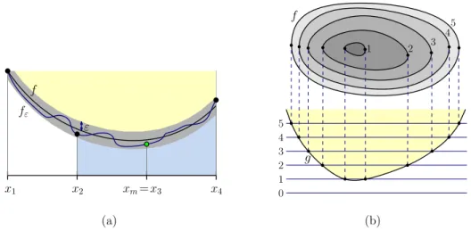
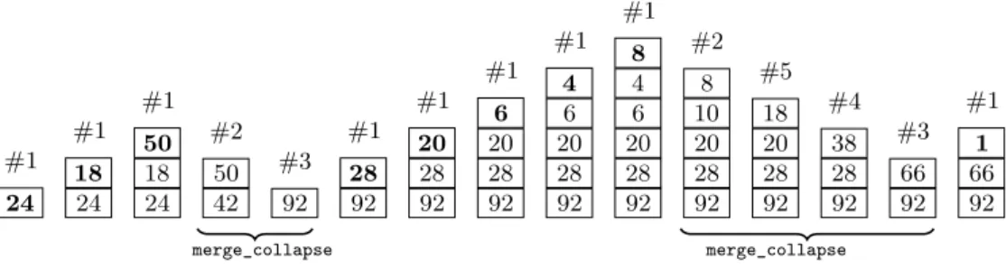
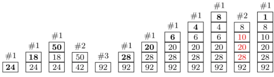
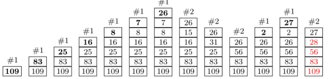
For each possible height 0 We use the vertical squares preprocessing data structure described in step 3 of the preprocessing. It is further complicated by the fact that we don't know the v-period of the elements in H. However, preprocessing time and storage grow as the combinatorial complexity of the polytope increases on powerbd/2c. Given a set S of n points in Rd and an approximation parameter ε >0, it is possible to compute an ε-approximation of the width S in O(nlog1ε+ 1/ε(d−1)/2+α)time, where α is an arbitrarily small positive constant. It is possible to store information of constant size with each polytope, so that we can compute in constant time the aγ-fattening affine transformation for the Minkowski sum of two polytopes from the collection. Applying Lemma 9, we can use this polytope to compute the aγ-fattening affine transformation forKi0⊕Kj0 in constant time, where γ= 1/(λ√ . d) = 1/d2. This information can be computed in time proportional to the size of the input polytope. According to Lemma 7, such hyperrectangles exist and can be computed in time proportional to the size of the input polytope [23]. Otherwise, we start by cutting the interval [a, b] and evaluate fε(x) at the four endpoints x1, x2, x3, x4 of the subintervals (see Figure 3(a)). If the minimum is within the interval [xm−1, xm+1], the recursive call will provide a value result through an inductive argument. We will consider the case where the input polytopes are represented by half spaces at the end of the next section. The case where the input is represented by dots is a trivial case of Theorem 2, where B ={O}. Nicolas Auger Vincent Jugé Cyril Nicaud The first version of the algorithm contained a bug, which was noted in [5]: while the input was correctly sorted, the algorithm did not behave as announced (due to a broken invariant). On the contrary, Java developers chose to stick with the first version of TimSort, and adjusted some tuning values (which depend on the broken invariants; this is explained in Sections 2 and 5) to avoid the error by [5 ] be exposed. The first feature of TimSort is working on the natural decomposition of the input string into maximum runs. Note that the stack height limit is not enough to justify TimSort's O(nlogn) runtime. Indeed, the calculation of the run decomposition (line 1) can be done immediately, by a greedy algorithm, in time linear inn, and the final loop (line 11) can be performed in the main loop by a fictitious run of lengths+ 1 to add. the end of the dissolution. Lethmaxbe the maximum number of runs in the stack during the entire execution of the algorithm. First, consider the sequence of cases #1 through #5 that are fired during the execution of TimSort's main loop. The following lemma points out one of the main reasons why TimSort is so efficient in terms of the number of runs. At any time during the main loop of Java's TimSort if the stack of runs is (R1,. At any time during the main loop of Java's TimSorton an input of size if the stack is (R1,. However, we prove that they hold ifi+ 2 andi+j+ 2 are not hindrance indices and ifi+j+ 1 is a hindrance index. It turns out that the constants and the expansion function mentioned in the proof of Proposition 11 are constructed as least fixed points of non-decreasing operators, although this construction should not have been obvious for the use of these constants and the function. Packing János Balogh József Békési György Dósa Leah Epstein A container is an array of elements of one class (in the division of potential inputs into elements of similar size, called classes), and can be complete if its intended number of elements has already arrived, or incomplete otherwise (but treated in the same way in both cases). The case when < 23 is more interesting, since a negative container with one element of size (13,12] and a positive container with one element of size above 12 can be packed into one bin if the total size of both objects does not exceed 1 (i.e. the volume their containers are the exact sizes of these two objects). The algorithm is defined for each step, based on the class of the new item. For a positive container with volume in the interval (1/2, a), the required weight of the container is indicated etc. Tree Decompositions Max Bannach The remaining work - computing a suitable optimized tree decomposition and performing the actual running of the dynamic program - is done by Jdrasil. To describe dynamic programs over tree decompositions, it seems useful to transform a tree decomposition into a more structured one. However, there is a pitfall: For each node, we must compute the set of potential states of the automaton depending on the sets of potential states of the children of that node, which leads to a quadratic dependence on|Q|. However, transitions of the form (qi, qj, ι(x), p) are difficult, since we now have to merge two sets of states. This already wraps up the description of the interface, everything else is done by Jdrasil. The result of this procedure is the StateVector object mapped to the root of the tree parse. The solid lines represent the actual decomposition edges, while the dashed lines illustrate the path (ie, some bags are skipped). Note that when we forget the vertexv, multiple states can become identical, which is handled here by the implementation of the JavaSet class, which automatically takes care of duplicates. Sp), or conclude that S is not a model for φ for any assignment of the free variables. Xq and bits required for optimization, and in the "asymmetric" ones of all other elements of the formula. 1600 D-Flat Jdrasil-Coloring Jatatosk Sequoia. b) Comparison of solvers for the 3-color problem on the full data set. c) The left picture shows the difference of Jatatoska vs. D-Flat and Sequoia. The right image shows the number of cases that can be solved by each of the solvers in seconds, i.e. -Flat Jdrasil-Coloring Jatatosk Sequoia. a) Mean, standard deviation, and median time (in seconds) each solver took to solve the 3-coloring across all instances of the dataset. Fomin, Lukasz Kowalik, Daniel Lokshtanov, Dániel Marx, Marcin Pilipczuk, Michal Pilipczuk and Saket Saurabh. Parameterized algorithms. Protocols for Community Detection Luca Becchetti Andrea Clementi Pasin Manurangsi Emanuele Natale Francesco Pasquale Prasad Raghavendra In this respect, any clustering strategy (like the one in [12]) which constructs (and then operates on) a static, sparse subgraph of the underlying graph is infeasible in the opportunistic model we consider here. Due to space limitations, most of the technical results are given in the full version of the paper [2]. Our first contribution is an analysis of the expected evolution of the averaging process over (n, d, β)-near regular graphs that possess a hidden and balanced partition of the nodes with the following properties: (i) The cut separating the two communities containo(m) edges; (ii) the subgraphs induced by the two communities are expanders, that is, the gapλ3−λ2. Over a suitable time window of length Ω(nlogn), the sign of the expected value of a node reflects the community to which it belongs, i.e. sgn. Our analysis of the process induced by Mean(1/2) provides the following bound, the proof of which can be found in the full version [2]. More formally, Corollary 7 below shows how such a global bound can be used to derive pointwise bounds on node values. The main idea of his proof is to first show that, with probability strictly greater than 1−ε, the number of ε-good nodes is at least n·(1−ε/logn) in each circle t∈[t1,2t1]. For any constant ε > 0 and for any λ3 > λ2 there exists δ depending only on ε and λ3 − λ2 such that for any sufficiently large n and for any ∈ [Ωε, λ3 − λ2 (nlogn), O ( n2)] applies to Prx (0), E. Note that the "good" time window begins after O(nlogn) rounds: so if the underlying graph has dense communities and a sparse cut, nodes can collectively compute an accurate label before the global mixing time of the graph. Importantly, the cost of our first protocol does not depend on the cardinality of the edge setE. The problem with the modified protocol above is of course that, in our setting, each vertex does not know the global time t. It is easy to see that after (nd/b) steps of our protocol, the 1−o (1) part of the values remains the same. Amariah Becker Philip N. Klein As we describe in more detail in Section 5, our PTAS for Bounded Capacity Vehicle Routing first applies Theorem 4 as the depot en0=/c for a constant to be determined, and obtains an embedding of the original graph in the bounded- tree-width graph H. The algorithm finds an optimal solution for this instance, and converts it to a solution for the original instance. Kachay gave a PTAS on Rd requiring Qto beO(log1/dlogn) [30], and Hamaguchi and Katoh [27] and Asano, Katoh and Kawashima [7] focused on constant-factor approximation algorithms for the case when the graph is a tree and customer request is separable. Feldmann et al.[20] observed that a shortest path cover for the scale naturally defines a clustering of vertices in cities[20]. D is a valid tree decomposition of H. 1 . ε), where θ is a limit on the doubling dimension of the sets XT. Since the size of the pockets is clearly bounded by the depth times the maximum cardinality of ˆXT, it suffices to prove that, for each cityT, ˆXT is bounded by (1ε)θ, and that the decomposition of the trees has a depthO( logc. Depending on this, their remaining two cases: whether it is connected to ˆh (see Fig. 4a) or not (Fig. 4b). First, if v is connected to a ˆin host graph, then dH(v,ˆh) =dG(v,ˆh) (and the same is true for u). Since X0k ⊆Bs(2k), the longest distance between two hubs is also at most 2·2k, therefore X0k has an aspect ratio of at most 2ε. The bound used in Lemma 13 on the cardinality of a set using its aspect ratio and its doubling dimension completes the proof. Polynomial-time approximation schemes for k-centered and capacity-constrained vehicle steering on finite-dimension freeway metrics. Proceedings, Part II, of the 42nd International Colloquium on Automata, Languages and Programming (ICALP), pages 588–600. The goal of the cop player is to catch the robber, ie. move at least one cop to the point occupied by the robber. The study of the Cops and Robbers game was started in 1978 by Quilliot [27], and a few years later it was independently introduced by Nowakowski and Winkler [7]. In the same work, they showed that a directed version of the game, without specifying initial positions, is also EXPTIME-complete. In addition, for an excellent survey of the results of the game, we refer the reader to the book by Bonat and Nowakowski [7]. Small nodes correspond to assignments of partial truths and are connected to the nodes of the clauses that satisfy them (ie, the corresponding literal is contained in those clauses). In the Cops and Robbers game on Gwith g cops, the cops have a winning strategy if it is satisfactory. a) Subgraph B can be seen as a set of vertices/points and lines on the plane. Conditional on the exponential time hypothesis, the problem of determining whether the graph number of a vertex N is at most tig(N) cannot be solved in time 2o(g(N)). Therefore, if the problem of determining whether the piece count of a vertex graph N is at most tig(N) can be solved in 2o(g(N)) = 2o(n)time, we can determine the satisfiability of φˆin poly( n) 2n·2o(n)= poly(n)2(+o(1))n time. Yixin Cao B. Sandeep We believe that H-free edge modification problems that admit polynomial kernels are exceptions. We assume that edge modification problems without H, when H is a claw or a paw, admit polynomial kernels. A vertex is in a maximal clique of type iif and only if it is contained in an induced diamond. Let E± be a minimal solution to an instance (G, k), and let K be a maximal clique of type iiinG. If K contains a protected node x that does not appear in any other type maximal clique from G, delete it. Since Rule 3 does not apply, every node in K is either a vulnerable node or a secure node in more than one large type maximal clique. As demonstrated in Figure 2, an edge can be deleted from a maximal clique of type ii. We show that every maximal clique of G∗ containing as a maximal clique of Gand is of type iiinG∗. Therefore, every maximal clique of G∗ containing x is a maximal gas well clique, i.e. of typeii in G∗. Dichotomy results on the hardness of edge modification problems without H. SIAM Journal on Discrete Mathematics. Massive Networks using Global Curveball Trades Corrie Jacobien Carstens Michael Hamann Ulrich Meyer Manuel Penschuck Hung Tran Although simple models such as Erdős-Rényi plots [11] are easy to generate and analyze, they differ too much from commonly observed power-law degree sequences. In turn, large benchmark graphs are required to evaluate the algorithms' scalability - in terms of speed and quality. External-Memory Model For example, consider the Fibonacci sequencex0= 0, x1= 1, xi=xi−1+xi−2∀i≥2, where each nodevi withi≥2 depends on exactly its two predecessors (see Fig. 1). The TFP technique achieves this as follows: as soon as xi has been computed, messages of the form hvj, xiii are sent to all successors (vi, vj)∈E. Edge-Switching Simple undirected curveball randomizes a graph by repeatedly selecting a pair of nodes {i, j} and permuting uniformly distributed neighbors at random. Its Markov chain is uncrossable, aperiodic and symmetric and therefore converges to the uniform distribution [6]. For the first two properties, it suffices to show that when a single trade from stateAtoB exists, there also exists a global trade from AtoB (see [4] for a similar argument).4 Note that there is a probability that is not zero, so that a single trade does not change the graph, e.g. In this case, a global trade degenerates into a single trade and the irreducibility shown in [4] persists. Initially, we send each edge to the earliest transaction in which one of the endpoints is active.6 In this way, the first transaction receives one message from each neighbor of the active nodes and can thus reconstruct Au1 and Av1. Thus, for each node (actively or passively) traded, the algorithm requires the index of the next transaction in which it is actively processed. We compare a series of uniform (single) trades, global trades and random switching and visually align the results of these schemes by defining asuper step. However, the effect is limited and in all cases performing 4 global trades for each rand link super step gives better results. We have omitted an in-depth discussion of single trades, preferring to focus on global trades that consistently outperform the former (cf. Section 3.2). All Curveball algorithms significantly outperform their direct competitors—even when we pessimistically performed two global trades for each edge-switching superstep (see Section 5.1). Verification of uniform sampling of binary matrices with fixed row sums and column sums for the fast curve algorithm. A fast and unbiased procedure to randomize binary ecological matrices with fixed row and column totals. Logarithmic Read Complexity Diptarka Chakraborty Debarati Das Michal Koucký Fredman [20] extended the definition of Gray codes to consider codes that may not enumerate all strings (although they were presented in a slightly different way in [20]) and also introduced the notion of a decision assignment tree (DAT) to study complexity any code in the bitprobe model. However, each of these constructs in the worst case reads n coordinates to create the next element. To increase the length of the C0 cycle in Zn+r2, we need to decrease k, the number of 2-functions in the decomposition. In the rest of the paper, we only present the constructions of the successor function nextt(C, w) for our codes. Construction of Gray codes 3 Chinese Remainder Theorem for Counters In the next two sections we describe the construction ofσ1, · ·, σk ∈ SN where=for somen∈N and how the value of depends on the length of the cycleσ=σk◦σk−1◦· · ·◦σ1. Such a matrix exists, for example, takeAto be the matrix of a linear transformation that corresponds to multiplication from the left of a fixed generator of the multiplicative group of Fqn under the standard vector representation of elements of Fqn. There exists a quasi-gray code on the domain(Fq)n+rof lengthqn+r−qr which can be implemented using a decision assignment treeT such that READ(T)≤r+ 2 and WRITE(T)≤2. Anish Mukherjee Venkatesh Raman To our knowledge, this has not been done before in the literature. In the implicit model, we use the classic bit encoding trick used in the development of implicit data structures [51]. The lex-DFS problem (both in undirected and directed graphs) is P-complete [54], and therefore polylogarithmic space algorithms are unlikely to exist in the ROM model. We discuss the lex-DFS algorithm for the directed graphs in the full version of the article [21]. When we go back to the top, we find the next white point (as in step forward) and continue until we have explored all the Gara points. It is easy to see that at most two full rotations of each list can occur during the execution of the algorithm (the first to explore all white neighbors and the second to find that there are no more white neighbors), resulting in a linear time lex -Algorithm DFS. Proof of Theorem 1(c) for undirected graphs Then any algorithm running in t(m, n) time in the rotational model can be simulated in the implicit model in (i)O(D·t(m, n)) time when G is given in the adjacency list, and (ii) O( lgD·t(m, n))time when Gi is given in the adjacent field. Furthermore, let rv(m, n) denote the number of rotations in v's list (of degree dv), and f(m, n) be the remaining number of operations. During preprocessing, for each vertex with degree at least 3, we ensure that the second and third elements of its neighbor list encode bit 0 (to mark it unvisited). For a vertexv with degree at least 3, we bring up its parent and swap the second and third elements to mark the node as visited (as before) when it is visited for the first time. We maintain the invariant that for any vertex with degree at least 3, as long as it is not visited, the second and third elements in its adjacent array encode the bit 0; and after the vertex is visited, its parent (in the DFS tree) is at the front of its adjacency array, and the second and third elements in its adjacency array encode the bit 1. So, when we visit a nodev with degree at least 3 for the first time, we bring its parent to the front, and then swap the second and third elements in the adjacent list, if necessary, to mark it as visited.5 Algorithm to Find 2D Maximal Repetitions
Applications to Width and Minkowski Sums
2 Preliminaries
Fattening
Projective Duality and Width
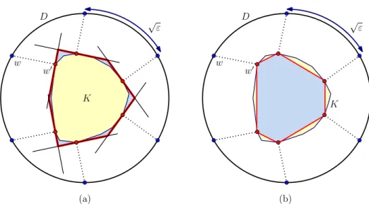
3 Approximate Convex Intersection
Convex Minimization
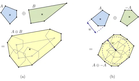
4 Minkowski Sum Approximation
Carine Pivoteau
2 TimSort core algorithm
3 TimSort runs in O(n log n)
4 Refined analysis parametrized with the number of runs
5 About the Java version of TimSort
6 Conclusion
Asaf Levin
2 Algorithm AH
Sebastian Berndt
3 An Interface for Dynamic Programming on Tree Decompositions
The Tree Automaton Perspective
The Interface
Example: 3-Coloring
4 A Lightweight Model-Checker for a Small MSO-Fragment
5 Applications and Experiments
6 Conclusion and Outlook
Luca Trevisan
3 First moment analysis
4 Second Moment Analysis
Second moment analysis for sparse cuts
Second moment analysis for dense cuts
5 Distributed Community Detection
The Sign-Labeling protocol for sparse cuts
The Jump-Labeling protocol for dense cuts
David Saulpic
New metric embedding results
Related Work
3 Embedding for Graphs of Bounded Aspect-Ratio
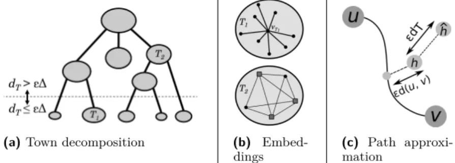
4 Main Embedding: Proof of Theorem 4 4.1 Embedding Construction
Proof of Error Bound
Tree Decomposition
5 Capacitated Vehicle Routing
PTAS for Bounded Highway Dimension
Sebastian Brandt
3 Preliminaries
4 The Construction
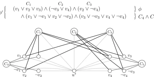
5 Hardness of Finding the Cop Number
Ashutosh Rai
Junjie Ye
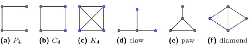
2 Maximal cliques
3 The kernel
Maximal cliques of type i
Maximal cliques of type ii
4 A cubic kernel for diamond-free edge deletion
Dorothea Wagner
2 Preliminaries and Notation
TFP: Time Forward Processing
3 Randomisation schemes
Simple Undirected Curveball algorithm
Undirected Global Trades
4 Novel Curveball algorithms for undirected graphs

5 Experimental Evaluation
Mixing of Edge-Switching, Curveball and Global Curveball
Runtime performance benchmarks
6 Conclusion and outlook
Nitin Saurabh
Related works
Our technique
4 Permutation Group and Construction of Counters
5 Counters via Linear Transformation
Construction of the counter
Srinivasa Rao Satti
2 DFS algorithms in the rotate model
Proof of Theorem 1(a) for undirected graphs
Proof of Theorem 1(b) for undirected graphs
3 Simulation of algorithms for rotate model in the implicit model
4 DFS algorithms in the implicit model – proof of Theorem 2
5 Concluding remarks