Eric Allender, Rutgers University Paul Beame, University of Washington Eric Blais, University of Waterloo Mark Braverman, Princeton University. Sevag Gharibian, University of Paderborn and Virginia Commonwealth University Shachar Lovett, University of California, San Diego.
Random Walks
1 Introduction
- PRGs and fractional PRGs
- Fractional PRG as steps in a random walk
- Polarization and fast convergence
- PRG for functions with bounded Fourier tails
- PRG for functions which simplify under random restriction
- Fourier tails of low degree F 2 polynomials
- PRGs with respect to arbitrary product distributions
- Related works
- Open problems
- Early termination
- Less independence
- More applications
- Gadgets
- Low degree polynomials
- Paper organization
We show that if X is a partial PRG for such F, then it can be used to approximate f(α) for any α∈[−1,1]n. Our current applications arise from the construction of a fractional PRG for functions with bounded Fourier tails.
2 General framework 2.1 Boolean functions
Pseudorandom generators
As discussed above, we wonder if our techniques can be used to construct a PRG for low degree F2 polynomials. We try to partially answer the question related to early termination of the random walk in Section 7.
Polarizing random walks
For this purpose, we need to apply some non-trivial conditions on the fractional PRG. We require that for each coordinate i∈[n], the value eXi is non-zero with appreciable probability.
3 Proof of Amplification Theorem
Proof of Lemma 13
We prove Lemma 13 in this section. Xt) is a partial PRG for F with errorsεt, and that it is (1−q) evident. The claim now follows from Claim 15. Xt) is a partial PRG for F with slightly worse error.
Proof of Lemma 14
J To provide some intuition that explains the rapid convergence of this random walk, note that once Ci becomes small enough, it becomes increasingly difficult to increase the value of eCi again. In other words, once we approach the boundary {−1,1}, the random walk converges faster as it becomes harder to move away from the boundary.
4 PRGs for functions with bounded Fourier tails
Applications
- Functions of bounded sensitivity
- Unordered branching programs
- Permutation branching programs
- Bounded depth circuits
There is an explicit PRG that foolsBn(w) with errorε >0 whose seed length is O(log(n/ε)(log logn+ log 1/ε)(logn)2w). There is an explicit PRG that fools n-variate functions computable by AC0 circuits of size and depth d, with error ε >0, whose seed length is O(log(n/ε)(log logn+ log 1/ε) log2d−2s).
5 PRG for functions which simplify under random restriction
6 Spectral tail bounds for low degree F 2 -polynomials
The proof now proceeds by noting that the above bound holds for any choice of y and z, and.
7 Smoothness
Bounded sensitivity functions
It is easy to check that this choice of (a, c) satisfies the required conditions, and completes the proof. A tight ω (loglog n) time bound for parallel rams to compute non-generated Boolean functions.
Sankeerth Rao
- Background and importance
- Prior Work
- Our results and merits of the paper
- Proof overview with an outline of key technical ideas used
- Stretch t pure bits to m pure bits,
- Stretch m pure bits to n pure bits,
- Overview of the paper
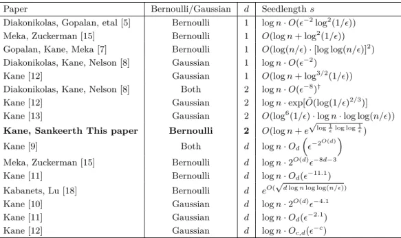
The best known constructions for PTFs of Boolean degree 2 use a starting length of s= logn·poly(1), the current work improves this, especially the error dependence tos=O(logn+subpoly(1)). The Meka-Zuckerman PRG for LTFs in [15] uses a similar idea of dimensionality reduction to reduce the seed length from O(log2(n)) to O(logn+ log2 1). Note that this significantly improves the seed length and the dependence on the error is additive and only grows subpolynomial, unlike the .
2 Preliminaries
- Basic results on polynomials, concentration, anticoncentration, invariance and regularity
- Eigenvalues of polynomials, Central Limit Theorem
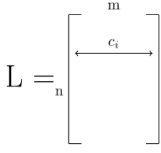
- Definition of L and basic facts
- Technical Lemmas involving L
After all parameters are fixed, we finally choose m= Ω(1)1 large enough so that all errors are bounded by O(). In the next lemma we show that they preserve L2 norms and internal products of vectors to give an idea of the kind of computations we need.
3 The regular case
Gaussian PRG | E
The main idea is that to figure out the average sign of a degree 2 polynomial, you just need to keep track of a few leading eigenvalues and the total measure over the rest of the eigenvalues. Thus, let's think of polynomials as few leading eigenvalues and a large amount of the rest of the eigenvalues.
Replacement for pL | E
- Linearize pL to pL lin
- Replacement for pL lin
Now this follows by noting that it approximately preserves the norms and inner products of vectors and that sinc is a constant that we can integrate. We now return from the Gaussian to the Boolean setting to complete the analysis for regular polynomials.
4 Reduction to the regular case
Leaf change
Changing Ly overall
- Changing from Ly 0 to Ly overall
- Changing Ly on leaves to Ly 0
Note that Ly and Ly0 agree everywhere except the hash variables collide with the decision path variables. A structure theorem for anticoncentrated weak Gaussian chaos and applications to the study of polynomial threshold functions.
Two-Source Extractors
- Extractors and Entropy-Rate Half
- The CZ Approach
- Our Main Result
- Our Technique
- Related work
- Random Variables, Min-Entropy
- Extractors
- Dispersers
The above query raises the question of what the dependence of the seed length of non-ejectable extractors is on the non-ejectability parameter. In Section 3, we demonstrate how the dependence of the seed on the length ont affects the parameters of the two-source extractor construction.
3 The Construction 3.1 The Overall Structure
- The Activation Threshold
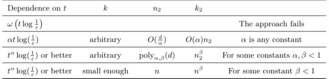
- The analysis fails when d ≥ ct log( 1 ε ) for some constant c
- When d = O(t log( 1 ε ))
- When d = O(t α log( 1 ε ))
A careful examination of the parameters shows that if the dependence on d1 ontis better, our scheme yields a two-source extractor that supports even smaller min-entropies. In Proceedings of the 53rd Annual IEEE Symposium on Foundations of Computer Science (FOCS), pages 688–697.
A The dependence of the seed on the non-malleability degree
To see why the Q's are not independent, consider for example the case where t= 2 and y is such that f2(f1(y)) =y. Depending on the arbitrary choice of the value of E for all points except (x, y), we denote them by e1,.
Polynomials and Subspace Designs
Chaoping Xing
- Our results
- Our approach
- Previous work
- Property T
- Monotone expanders
- Rank condensers
- Organization
Moreover, our paradigm is flexible enough to allow the construction of unbalanced dimension expanders. Thus, we have reduced the task of constructing dimension expanders to the task of constructing subspace models.
2 Background 2.1 Notation
Dimension expanders
In section 2, we set notation and define the various pseudorandom objects that we use in our construction. The collection {Γj}dj=1 forms a b-unbalanced(η, β)-dimensional expansion if for all subspaces U ⊆FN of dimension at most ηN,.
Subspace design
Hk ⊆V afFq subspace is called a (s, A, d)-subspace design inV if for every Fqd subspaceW ⊆V afFqd dimension s,. In previous works, what we have called an (s, A, d) subspace design would have been called an (s, As, d) subspace design.
Periodic subspaces
We call a subspace design explicit if there exists an algorithm that derives the bases Fq for each subspaceHi in the poly(n) field operations.
3 Dimension expander construction
Construction
Analysis
4 Constructions of subspace designs
Subspace designs via an intermediate field
Construction via correlated high-degree places
5 Explicit instantiations of dimension expanders
6 Conclusion
Explicit list-decodeable rank-metric and subspace codes via subspace designs.IEEE Transactions on Information Theory. Black box polynomial identity test of generalized depth-3 arithmetic circuits with bounded top fan-in.
OR-AND-MOD Circuits
Igor C. Oliveira
Rahul Santhanam
The Minimum Circuit Size Problem
Note, however, that the Kabanets–Cai result does not provide any evidence against the NP-hardness of the MCSP—it only suggests that the NP-hardness may be difficult to establish. There have been a number of works that build on this result to provide further proof of the difficulty of showing NP-hardness of MCSP.
Our Result
As argued in [14], top fan-in is the preferred metric for OR-AND-MOD2 circuits, because: (i) it measures the number of affine subspaces needed to cover the 1s of the function, and therefore has a nice combinatorial meaning; (ii) using basic linear algebra, the number of MOD2 gates input into a middle layer AND gate can be assumed to be at most n without loss of generality, and thus the top fan-in approximates the total number of gates to within a radius factor n; and (iii) the size of a DNF is often measured by the number of terms in it, and analogously it makes sense to measure the size of a DNF of Parities by the top fan-in of the circuit. Can we prove lower bounds against proof systems whose lines are encoded by circuits in the class.
Overview of the Proof of Theorem 1
Using this construction, we are able to show by delicate analysis that if t is sufficiently large, the following holds with high probability: ifS admits a covering of size K, then DNFXOR(f)≤K; moreover, if DNFXOR(f)≤K, then S allows a cover of size ≤2K. We discuss the intuition for this claim in Section 3.1.) This construction and the hardness of approximation result forr-Bounded Set Cover imply that (DNF◦XOR)-MCSP∗ is NP-hard under many-one randomized reductions. Again, a careful argument allows us to establish the following relation between the partial function f and the total function g: with high probability over the choice of the random linear subspaces (Lx)x∈f−1(∗),DNFXOR(g) = DNFXOR(f) +|f−1(∗)|. We discuss the intuition for this claim in Section 3.2.) Consequently, it follows from this and the previous reduction that (DNF◦XOR)-MCSP is NP-hard under many-one randomized reductions.
Circuit Size Measure and Its Characterization
That means, there are coefficients1k,. atk∈Zmand an element bk ∈Zms such thatPt. i=1aikxi=bk if and only ifCk accepts input x. k=1Ck admits the intersection of such linear equations over Zm. Since X is not empty, we can get some elementsx0∈X. Now, we can rewrite X as Indeed, for a vector b := Aa, we have X=H+a={x∈Ztm|Ax=b}; so we can construct an AND◦MODmqark that accepts.
Computational Problems
We present a reduction of a 2-factor approximation of the r-bounded set covering problem to (DNF◦MODm)-MCSP∗. We will prove that (vi)i∈[n] is nice with probability at least 12, and that for any nice (vi)i∈[n], the minimum size of DNF◦MODm is a 2-factor approximation of the minimum is set cover size.
Derandomizing the Reductions
The random reduction of Theorem 16 can now be derandomized using the deterministic construction of Theorem 25 zar:=t+ 2. We generate random vectors using the pseudorandom generator for AND◦MODm circuits and show that the probabilistic argument of claim 14 still works.
Near-Optimal Pseudorandom Generators for AND ◦ MOD m
Thatcher, editors, Proceedings of a symposium on the Complexity of Computer Computations, held in March at the IBM Thomas J. Miller, editor, Proceedings of the Twenty-Eighth Annual ACM Symposium on the Theory of Computing, Philadelphia, Pennsylvania, USA, pages May 435–441.
B On Different Complexity Measures for DNF ◦ MOD p Circuits
We can see that ϕ is a homomorphism; thus it suffices to prove that the kernel of ϕ is only 0∈V⊥. Then the smallest number of gates in any layeredAND◦MODp formula that accepts A is exactly 1 + codim(A).
C A Hardness of Approximation Result for (DNF ◦ MOD m )-MCSP
First, note that to conclude this it suffices to describe a quasipolynomial-time algorithm B that approximates the cover of the r-bounded set within a factor γlogr(n) for r(n) = logn. Then the Feige reduction product is an example of the set cover problem onN :=m(5n)`.
Linear Combinations of Simple Functions
Thresholds, ReLUs, and Low-Degree Polynomials
Intuition
Here we provide an overview of some of the ideas used to prove lower bounds in this work. Therefore, there exists a natural barrier to proving the lower bounds of exponential sparsity for linear combinations of polynomials of “slightly low” degree.
3 Meta-Theorem for Lower Bounds on Linear Combinations of Simple Functions
Lower Bounds for Exponential Time With an NP Oracle
Then there is a function iENP that does not have SUM◦ C-circuit with sparsity2αn, for some α >0. There is an ε >0 and an O(2n−εn) time algorithm for computing the Sum-Product ofk functions from C, and.
4 Sparse Combinations of Threshold Functions
Using the Sum-Product algorithm for assumption (A) running in O(2n−εn) time and setting α >0 to be sufficiently small, the running time iso(2n). Furthermore, for every unboundedα(n) such that nα(n) is time constructible, there is a function inNTIME[nα(n)] that does not have SUM◦THR circuits with polynomial sparsity.
5 Sparse Combinations of ReLU Gates
Using Theorem 10, each of the threshold functions [hx, wii ≥ −ai] can be represented as a linear combination of t = poly(n) exact threshold functions. A more efficient algorithm for the problem defined by (2) can be obtained by preprocessing the second half of the vectors (ie, the w0A0 vectors).
6 Sparse Combinations of Low-Degree Polynomials over Finite Fields
We first convert the sum-product problem of (3) to an equivalent sum where each "term" in the sum is a small system of polynomial equations. Converting to SUM◦MODp◦ANDdc, Theorem 26 says that the Sum-Product problem can be solved in 2n−n/O(dc) time (omitting low-order terms).
7 Conclusion
Super-linear gate and super-quadratic wire lower bounds for depth-two and depth-three threshold circuits. Circuit Lower Bounds for Nondeterministic Quasi-Polytime: An Easy Evidence Lemma for NP and NQP.
A Linear Lower Bound for AND With Sums of Quadratic Polynomials
Russell Impagliazzo
Valentine Kabanets
Ilya Volkovich
- Conditional collapses
- Interpretation
- Circuit lower bounds
- Interpretation
- Consequences for natural properties
- Obfuscation
- Interpretation
- Hardness of relativized versions of MCSP
- Our techniques
More specifically, they show that if any of the above classes have polynomial-sized Boolean circuits, the corresponding class collapses to MA, which is known to be in ZPPNP [7, 20]. Some of the proofs (for example, our proof that ⊕P has a complete problem that is both downward and arbitrarily self-reducible) are given in the appendix.
2 Preliminaries 2.1 Basics
- Derandomization from hardness
- Natural properties, PAC learning and MCSP
- Obfuscation
- Downward self-reducible and self-correctable languages
- Learning downward self-reducible and self-correctable languages
Let R be a strongly useful natural property and let L be a downward, self-reducible, and self-correctable language. Different complexity classes have complete problems that are both downward self-reducible and self-correctable.4.
3 The proofs
- Conditional collapses
- Circuit lower bounds for MCSP-oracle classes
- IO related results
- Hardness of relativized versions of MCSP
- PSPACE ⊆ ZPP MCSP PSPACE [2]
Suppose Boolean circuits are PAC-learnable using membership and B queries with hypotheses that are B oracle circuits. First we see that for each oracleB there is a PMCSPB natural property forB oracle circuits.
4 Open questions
In Proceedings of the 45th Annual IEEE Symposium on Foundations of Computer Science (FOCS), pp. A survey of Russian approaches to perebor (brute-force searches) algorithms.IEEE Annals of the History of Computing.
A Self-correctable and downward-reducible ⊕P-complete problem
Note that each bit j of the value fn,n(¯y) for each input ¯y is computable in P and thus also in ⊕P. The latter is exactly the jth bit of fn,i because the addition in the F2k field is the bitwise XOR of the corresponding one.
B Proof of Lemma 35
The downward decrease of F follows from the property of fn,i (and the way we arranged the lengthsh(n, i)). The parity of the number of receiving paths of the above algorithm is exactly the sum of the modulo 2 bits in all logical assignments toxi+1,.
5 It is easy to see that sketching over finite fields can be significantly better than linear sketching over integers for certain calculations. It can be found that the corresponding
Previous work and our results
Communication complexity
The one-way partition complexity down with respect to µ, denoted as Dδ→,µ(f) is the smallest communication cost of a one-way deterministic protocol that f(x, y) with probability at least 1−δ over the inputs ( x, y ) drawn from the distribution µ. One-way communication complexity over product distributions is defined as D→,×δ (f) = supµ=µx×µyDδ→,µ(f) where µx and µy are distributions overFn2.
Fourier analysis
We say that a deterministic protocol M(x) with the length of the message that Alice sends to Bob divides the rows of this matrix into 2tcombinator rectangles where each rectangle contains all the rows of Mf corresponding to the same fixed message ∈ {0,1}t .
3 F 2 -sketching over the uniform distribution
The following lemma bounds the error probability of the one-way protocol from below in terms of the excluded Fourier coefficients and the conditional distribution of the different parities of Alice's input conditional on Alice's random message. For any fixed message m sent to Alice, let Dm denote the distribution of Alice's input x conditional on the event that M = m.
4 Applications
- Low-degree F 2 polynomials
- Address function and Fourier sparsity
- Symmetric functions
- Composition theorem for majority
Clearly, any linear combination of more sets than M has a Hamming weight greater than the contribution of the first dcoordinates. This means that every non-trivial linear combination of M rows contains a 1 in one of the first t coordinates.
5 Streaming algorithms over F 2
Random streams
Combining Theorem 31 and Lemma 29, we have that any set of vectors dominated by O(S) for some standard subspaceSsatisfiesP. The proof follows directly from Theorem 4 since in both models we can divide the current intoσ1 andσ2 so that freqσ1 and freqσ2 are both uniformly distributed over Fn2.
Adversarial streams
The same argument implies that the transition function of a path-independent automaton must be linear since (x+y)∗o=x∗(y∗o). Tight bounds on the randomized communication complexity of symmetric XOR functions in one-way and SMP models.
A Information theory
Proof of Fact 16
B Deterministic F 2 -sketching
Disperser argument
Composition and convolution
Multiplication of all these multilinear expansions corresponding to the term ˆf(S)χS gives a polynomial which is a sum of at most bn monomials where the number of non-zero Fourier coefficients is ofg. Each such monomial is obtained by choosing one monomial from the multilinear expansions corresponding to different variables in χS and multiplying them.
C Randomized F 2 -sketching