Numerical investigations of lateral tidal straining in regions of freshwater influence in the German Bight with the one ‐ dimensional GOTM model
Master Thesis
M.Sc. Program for Polar and Marine Sciences POMOR
Supervisors: Prof. Dr. Hans Burchard PD Dr. Christian Winter Prof. Dr. Victor Ionov
Saint Petersburg State University / Hamburg University By Vladislav Onopko
August 28, 2017
Numerical investigations of lateral tidal straining in regions of freshwater influence in the German Bight with the one ‐ dimensional GOTM model
Vladislav Onopko
Master Program for Polar and Marine Sciences POMOR / 022000 Ecology and environmental management
Supervisors:
Prof. Dr. Hans Burchard, Leibniz Institute for Baltic Sea Research Warnemuende, Germany
Dr. Christian Winter, MARUM Center for Marine Environmental Sciences Bremen, Germany
Prof. Dr. Victor Ionov, Saint Petersburg State University, Russia
Abstract
This Master thesis deals with numerical investigations of lateral tidal straining in regions of freshwater influence (ROFI) in the German Bight, based on the ADCP data observations completed by the research center “Marum”. For this study, plots of the ADCP data were performed through MATLAB software. Simulation results of velocity magnitude, velocity direction, salinity and absolute shear were obtained by using the General Ocean Turbulence Model (GOTM) and interpreted through the programming language “Python”. Moreover, the sensitivity analysis of the density salinity gradient direction, its strength and tidal current velocity magnitude was achieved based on these GOTM simulation results. This analysis was completed to find a setup of the GOTM model that can or cannot reproduce the ADCP observations, obtaining that the best match coincides with a density salinity gradient of -1.6 × 10⁻⁴ psu m-1 directed from the south (α = 270°) and a tidal current velocity of 0.5 m s-1. In addition, this research determined the drivers and their dimensions, which influence on lateral tidal straining phenomenon.
Obtained results of this Master thesis contribute to further investigation of lateral tidal straining in the regions of freshwater influence as well as understanding the parameters that influence on the dynamic regime of the water column in coastal waters. According to the GOTM simulations these regimes can be: permanent stratification, strain‐induced periodic stratification (SIPS) and well mixed. All of them have a crucial role in controlling sediment transport and the vertical fluxes of water properties such as heat, salt and nutrient elements.
Численное моделирование горизонтальных приливных деформаций пресноводного стока в Немецкой бухте на одномерной модели GOTM (ГОТМ)
Владислав Онопко
Магистерская программа «Полярные и морские исследования» («ПОМОР») / 022000 «Экология и природопользование»
Выпускная квалификационная работа магистра Научные руководители:
Профессор Ганс Бурхард, Институт Изучения Балтийского Моря им. Лейбница в г. Варнемюнде, Германия
Доктор Кристиан Винтер, Центр Морских Наук об Окружающей Среде «Марум» в г. Бремен, Германия
Кандидат географических наук, доцент, Ионов Виктор Владимирович, Институт Наук о Земле, Санкт-Петербургский Государственный Университет, Россия
Абстракт
Данное исследование, выполненное в рамках выпускной квалификационной работы магистра, посвящено численному моделированию горизонтальных приливных деформаций пресноводного стока в Немецкой бухте основываясь на данных, полученных с океанографического измерительного оборудования ADCP в ходе экспедиции от центра морских наук об окружающей среде «Марум». В данной работе, графики, отображающие данные с ADCP оборудования, были получены путем интерпретации этих данных с помощью высокоуровневого языка и интерактивной среды для программирования, численных расчетов и визуализации результатов MATLAB. С помощью одномерной модели GOTM были смоделированы такие факторы как: сила течения и его направление в результате горизонтальных приливных деформаций пресноводного стока, соленость и абсолютный сдвиг течения в водной толще при определенных условиях.
Интерпретация и визуализация значений данных смоделированных факторов была выполнена с помощью языка программирования «Python». Также, был проведен систематический анализ с помощью одномерной модели GOTM возможных градиентов солености, его направлений и скорости течения прилива, данные о которых не были определены ADCP оборудованием в ходе экспедиции. Данный систематический анализ был выполнен для того, чтобы понять при каких
параметрах одномерная модель GOTM может или не может воспроизвести такие же результаты о динамических процессах в водной толще полученные с ADCP оборудования. Наиболее схожие результаты учитывают такие параметры как градиент солености равный -1.6 × 10⁻⁴ псю м-1, направленный с юга (α = 270°) и скорость течения прилива равная 0.5 м с-1. Более того, в ходе данного исследования были определены факторы и их размерность, которые вызывают горизонтальные приливные деформации. Полученные результаты в данной выпускной квалификационной работе магистра делают способствуют дальнейшему изучению горизонтальных приливных деформаций пресноводного стока, а также факторов, которые оказывают влияние на динамические режимы в водной толще прибрежных вод. Исходя из смоделированных результатов с помощью одномерной модели GOTM данными динамическими режимами могут быть: постоянная стратификация, вызванная деформацией пресноводного стока периодическая стратификация и отсутствие стратификации (перемешенный режим).
Динамический режим играет значительную роль в распределении наносов и вертикальном распределении таких важных факторов как тепла, солености и питательных элементов в водной толще.
Contents
Introduction ... 7
Material and methods ... 13
1.1 The study area ... 13
2.2 The one-dimensional water column model ... 16
2.3 One-dimensional analysis: one-dimensional dynamic equations ... 17
2.4 Simpson number ... 18
2.5 ADCP data ... 19
Results ... 21
3.1 Idealized one-dimensional GOTM model simulations ... 21
3.2 Density salinity gradient magnitude ... 22
3.3 Relative direction effect of the density salinity gradient ... 22
3.3.1 Relative direction of the density salinity gradient α = 0° ... 23
3.3.2 Relative direction of the density salinity gradient α = 45° ... 24
3.3.3 Relative direction of the density salinity gradient α = 90° ... 25
3.3.4 Relative direction of the density salinity gradient α = 135° ... 26
3.3.5 Relative direction of the density salinity gradient α = 180° ... 27
3.3.6 Relative direction of the density salinity gradient α = 225° ... 28
3.3.7 Relative direction of the density salinity gradient α = 270° ... 29
3.3.8 Relative direction of the density salinity gradient α = 315° ... 30
3.4 Sensitivity analysis of the density salinity gradient magnitude effect ... 34
3.4.1 Velocity direction response to the density salinity gradient moving from the south-west (α = 225°) ... 35
3.4.2 Velocity direction response to the density salinity gradient moving from the south (α = 270°) ... 36
3.4.3 Velocity direction response to the density salinity gradient moving from the south-east (α = 315°) ... 37
3.4.4 Salinity response to the density salinity gradient moving from the south-west (α = 225°) ... 39
3.4.5 Salinity response to the density salinity gradient moving from the south (α = 270°) ... 40
3.4.6 Salinity response to the density salinity gradient moving from the south-east (α = 315°) ... 41
3.5 Sensitivity analysis of the tidal current velocity magnitude ... 43
3.5.1 Response to the density salinity gradient = -1.6 × 10⁻⁴ psu m-1 moving from the south (α = 270°) and tidal current velocity = 0.3 m s-1 ... 44
3.5.2 Response to the density salinity gradient = -1.6 × 10⁻⁴ psu m-1 moving from the south (α = 270°) and tidal current velocity = 0.8 m s-1 ... 45
6
3.5.3 Response to the density salinity gradient = -2.0 × 10⁻⁴ psu m-1 moving from the
south-west (α = 225°) and tidal current velocity = 0.3 m s-1 ... 46
3.5.4 Response to the density salinity gradient = -2.0 × 10⁻⁴ psu m-1 moving from the south-west (α = 225°) and tidal current velocity = 0.8 m s-1 ... 47
Discussion ... 49
4.1 Comparison the GOTM simulation results to the ADCP data ... 50
4.2 Quantifying of tidal straining phenomenon by Simpson number ... 54
Conclusions ... 57
Acknowledgements ... 59
References ... 60
7
Introduction
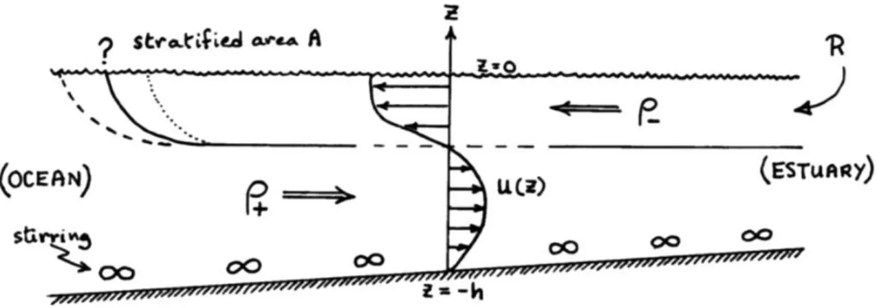
Tidal straining is a phenomenon of temporal variations in stratification and mixing resulting from the interaction of longitudinal density gradients with the horizontal tidal velocity. As a result, the theory predicts stronger and weaker stratification during ebb/low tide and flood/high tide, respectively. In more detail, this oceanographic process is represented in Fig.1, where freshwater input from rivers induces substantial horizontal gradients of density in estuaries and the surrounding waters. These density gradients drive a shear flow circulation with low-density water flowing offshore at the surface and higher density water moving shoreward at the bottom (Simpson et al. 1990).
Fig. 1. Schematic of a stratified region maintained by freshwater input in competition with bottom stirring. The estuarine circulation u (z) moves light water offshore at the surface and heavier water onshore in the lower layers thus increasing stratification (Simpson et al. 1990).
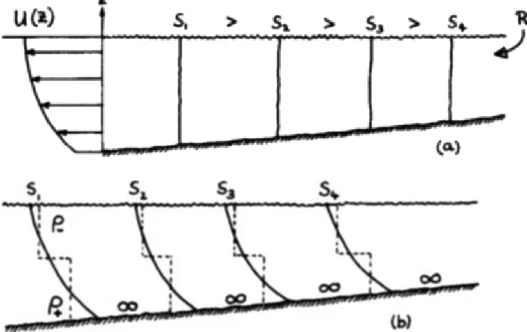
Furthermore, the shear acts on the horizontal density gradient to induce vertical structure by the mechanism illustrated in Fig. 2. Isolines of salinity, which are initially vertical at the start of the ebb, are distorted by differential displacement, with the lighter surface water moving faster seaward and overtaking heavier, more saline water in the lower layers and thus generating a stable structure. Vertical mixing by wind stress near the surface and tidal stress at the bottom will tend to transform the structure into a two-layer profile with a sharp halocline (Simpson et al. 1990).
8
Fig. 2. Schematic of tidal straining: (a) isolines vertical at start of ebb (b) stratification induced by shear on the ebb modified by top and bottom mixing (Simpson et al. 1990).
According to Simpson et al (1990) and Verspecht et al. (2009), three dynamic regimes can be observed in coastal waters tidal flows under the influence of horizontal density gradients: well‐mixed flow during the entire tidal cycle, alternation between stratified and well mixed stages (SIPS) and permanently stratified regimes. Furthermore, Simpson determined that a major parameter governing this tidal straining dynamics exists and is defined as the Simpson number, which has numerical relationship between the tidally averaged longitudinal buoyancy gradient ∂xb, the mean water depth and a scale for the bottom friction velocity (or tidal velocity amplitude U).
The presence of valuable salinity density gradients is common for the regions of fresh water influence for which this study is being conducted. However, for this master thesis was chosen the region of fresh water influence (ROFI), in the German Bight. Due to motivation by Acoustic Doppler Current Profiler (ADCP) data, which was obtained during the HE-417 expedition in the German Bight from the 13th of March until 18th of March in 2014 year and was organized by the research center “Marum”. The coordinates
of the area in the German Bight, where ADCP measurements were taken, are 53° 59 ̍ 28 ̍ ̍ N and 6° 52 ̍ 43 ̍ ̍ E. The ADCP data for the studied area is presented in
Fig. 3 as velocity direction and in Fig. 4 as velocity magnitude.
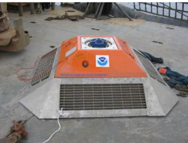
ADCP is an Acoustic Doppler Current Profiler (Fig. 5), which measures ocean currents and follows the premise of the Doppler effect, it emits a series of high-frequency pulses of sound that bounce off of moving particles in the water. If the particle is moving away
9
from the instrument, the return signal is at a lower frequency. If the particle is moving toward the instrument, the return signal is at a higher frequency. Because the particles move at the same speed as the water that carries them, the speed of the water’s current can be determined. The ADCP is usually equipped with four acoustic transducers that emit and receive signals from four different directions. This allows the instrument to measure currents at different depths simultaneously (NOAA's National Ocean Service:
Education Currents, 2007).
Fig.3. The image of the velocity direction (°) based on the ADCP data.
Fig.4. The image of the velocity magnitude (m s-1) based on the ADCP data.
10
Fig. 5. ADCP – an Acoustic Doppler Current Profiler (https://oceanservice.noaa.gov).
The region of fresh water influence (ROFI) is the region between the shelf sea regime and the estuary, where the local input of freshwater comes from the coastal source. The term region of fresh water influence (ROFI) was introduced by Simpson et al. (1993) as a generalization of the river plum terminology. The main feature of ROFI is that saltwater from the open ocean and freshwater from the land drainage, mix with each other under tidal and wind forcing, producing measurable salinity gradient in the horizontal direction (Prichard,1952; Cameron and Prichard,1963; Hansen and Rattray, 1965). In addition, river plumes can maintain their cross-shelf structure for hundreds of kilometers (Fong and Geyer 2001, 2002; Yankovsky et al. 2001). Consequently, they are extremely important in determining the transfer of matter and the fate of pollutants in coastal seas.
Furthermore, due to presence of tides and freshwater input, strain-induced periodic stratification (SIPS) can appear in the water column, in the region of freshwater influence (ROFI). Strain-induced periodic stratification (SIPS) is a certain balance between the tidal force and the density salinity gradient, when the water column may be stratified during ebb and flood and well mixed after these events (Simpson et al. 1990).
Understanding the development and break down of tidal straining is a key objective of coastal waters oceanography. The level of tidal straining leads to the appearance of stratification in the water column, which is crucial in controlling the vertical transport, for example, the vertical fluxes of water properties such as heat, salt and the nutrient elements. This last factor might be very important in controlling the phytoplankton growth rate and consequently, in limiting biological production. Furthermore, by inhibiting vertical displacement, stratification induced by tidal straining can change the degree of light penetration in the water column. This important element has influence on the distribution of phytoplankton in the water column. In case of strong stratification,
11
phytoplankton can obtain light energy only in shallow waters. On the other hand, in an environment where vertical mixing is complete, the phytoplankton has a possibility to transfer over the full depth.
Besides the horizontal dispersion of salt, nutrients, pollutants, and biological organisms, a major motivation for studying lateral tidal straining in regions of freshwater influence is its impact on the water circulation and therefore, sediment transport. Since many coastal regions contain important economical infrastructure like harbors or shipping routes, which have to be maintained by expensive sediment dredging, understanding the underlying mechanisms that accumulate sediments and move the water circulation in those areas is of large economical interest.
The main goal of this master thesis is to find and discuss a setup of the GOTM model that can (or cannot) reproduce the ADCP observations, obtained during the HE-417 expedition in the German Bight from the 13th of March until 18th of March in 2014 year, based on the General Ocean Turbulence Model (GOTM), which is a one-dimensional water column model for the most important hydrodynamic and thermodynamic processes related to vertical mixing in natural waters.
The GOTM simulations are a very useful numerical tool that has been widely applied for several studies in order to compute solutions for one-dimensional versions of the transport equations of momentum, salt and heat in the water column. For example, Hans Burchard et al. 2008 applied GOTM in order to study the impact of density gradients on the sediment transport into the Wadden Sea. In addition, Hans Burchard 2009, also applied the GOTM simulations to have a better understanding of the effects of wind, tide, and horizontal density gradients on the stratification in estuaries and coastal seas.
In this master thesis, the GOTM simulations are then applied to solve three problems main: determination of the tidal straining drivers, their dimensions that influence tidal straining occurrence and, subsequently, investigation of consequences induced by tidal straining.
This research was completed as a Master thesis for the Russian-German Master Program
"Polar and Marine Sciences". The text of the thesis is divided into Introduction, Material and Methods, Results, Discussion and Conclusions.
12
The following study is divided into three chapters, which first chapter gives a general description of the German Bight and its oceanographic characteristics, focusing on properties as temperature, salinity, density salinity gradient and tidal current velocities.
In addition, chapter 1 has a description of the numerical model developed along with information about the ADCP data obtained from the measurements during the HE-417 expedition in the German Bight. Furthermore, in this chapter a description of the one- dimensional dynamic equations used is given, outlining the appropriate formulas used by GOTM model for calculation particular values. Chapter 2 contains a sensitivity analysis of the model reaction to different strengths of the density salinity gradient and predict the effect of the relative salinity gradient direction. In addition, the analysis of different velocity magnitudes is included as a sensitivity parameter. Chapter 3 contains the interpretation of the results and describes the significance of this master thesis findings, what was already known about the research problem being investigated, and explain new understanding or insights about the problem. Finally, in the conclusions, highlights key points of analysis and results are provided. Moreover, this chapter shows new facts obtained in the investigation of tidal straining in the regions of freshwater influence in the German Bight and establish the importance of the research conducted within the framework of the Master thesis.
13
Chapter 1
Material and methods
1.1 The study area
The study is the region of fresh water influence in the German Bight (Fig.6). The circulation of German Bight is highly complex, characterized by strong tidal currents, rough bathymetry, energetic turbulence, and density gradients born of the competition between ocean and river waters. The depth-averaged tidal mean velocity ranges between 0.3 and 0.8 m s-1 (van Alphen et al. 1988). The topography of the German Bight is a result of the retreat of glacial ice cover and rising sea level during the last 10000 years (Becker, G. A. et al. 1992) and shows nearly rectangular coastline with a funnel-like 30 to 40-m deep (Stanev, E. V. et al. 2014).
Fig.6. The German Bight. The image is of Aqua/MODIS March 9, 2014, 11:50 UTC.
The German Bight is generally formed by two main water masses: continental coastal water and central (southern) North sea water (Becker et al. 1992). The central southern North sea water is divided into a surface layer and a bottom layer component, which is found in the post-glacial valley of the river Elbe. The continental coastal water which is a mixture of: water from the Atlantic, from the English Channel and from the rivers Rhine, Meuse and Ems (Becker et al. 1992).
14
The Rhine river is approximately 30-km-wide and 100-km-long region of freshwater influence at the southeast coast of the Southern Bight of the North sea along the Dutch coast (Souza and Simpson 1997). Due to the Coriolis force and the prevailing west and southwest winds, the Rhine plume is deflected northeastward and provides main freshwater input to the Dutch coastal current (Souza and Simpson 1966; de Ruijter et al.
1997).
The Ems is a river in the northwestern Germany. It discharges into the Dollart Bay, which is part of the German Bight and has a basin of 17,934 km2 (Van Leussen 1994).
Approximately, between Papenburg and Emden, the river is classified as brackish, though the brackish zone migrates through a 30 km stretch of river depending on freshwater flow (Talke and de Swart 2006).
The lower part of the Elbe is a partially mixed coastal plain estuary and has a river basin of 148,268 km2 (Scheurle et al. 2005). It is the largest estuary on the German coast of the North Sea. Also, Elbe estuary exhibits well developed turbidity maxima in the low salinity regions of the mixing zones between freshwater and saltwater. The large tidal range (4 m at spring tide) develops near the mouth of the Elbe. Tides are semidiurnal with a marked diurnal asymmetry (Jens Kappenberg and Iris Grabemann, 2001).
On the other hand, the Weser river also influences the salinity of the German Bight considerably. This influence is indicated by a near-coastal low-salinity plume. The Weser flows through Lower Saxony and then into the German Bight and has a basin of 46,306 km2. The roughly 130 km long estuary is strongly influenced by tides (Scheurle et al.
2005).
The physical properties in the German Bight as salinity, temperature and density are used to study interactions between them and their possible influence on the tidal straining phenomenon. Temperature measurements from March 2014 from the BSH agency are observed in Fig.7, where temperature of the German Bight ROFI ranges between 6 to 8°C. Data collected in the beginning of the 20th century (Fig.8) shows that the salinity varies from 26 psu to 34.5 psu in the German Bight ROFI. Finally, density values of the area are ranging from 1025 to 1027 kg m-3 (Fig.9).
15
Fig.7. Map of the sea surface temperature of the German Bight, from March 2014.
(Federal Maritime and Hydrographic Agency of Germany)
Fig.8. Map of the sea surface salinity of the German Bight, averaged for March from 1902-1954. (Federal Maritime and Hydrographic Agency of Germany)
16
Fig.9. Map of the sea surface density of the German Bight, averaged for March from 1902-1954. (Federal Maritime and Hydrographic Agency of Germany) 2.2 The one-dimensional water column model
The General Ocean Turbulence Model (GOTM) was used in this study. It is a one- dimensional water column model for the most important hydrodynamic and thermodynamic processes related to vertical mixing in natural waters. The core of the model computes solutions for the one-dimensional versions of the transport equations of momentum, salt and heat. This module contains the definitions of the most important mean flow variables such as the mean horizontal velocity components, U and V, the mean potential temperature Θ (or the mean buoyancy, B) and the mean salinity, S (Umlauf et al. 2010). The main advantage of GOTM in comparison with other 1D models is a powerful and abundant turbulence module. At least one turbulence model from each type is implemented into GOTM tree code (Umlauf et al. 2010).
Due to the one-dimensional character of GOTM, the state-variables listed above are assumed to be horizontally homogeneous, depending only on the vertical z-coordinate.
As a consequence, all horizontal gradients have to be taken from observations, or they have to be estimated, parameterized or neglected (Umlauf et al. 2010).
Another option in GOTM for parameterizing the advection of Θ and S is to relate the model results to observations. Evidently, this raises questions about the physical
17
consistency of the model, but it might help to provide a more realistic density field for studies of turbulence dynamics (Umlauf et al. 2010).
The GOTM program consists of several sections connected through a main core module called "gotm", which control the time-stepping management and initiate all other sections following a specific order. Between the modules of the program, the "meanflow"
calculates water properties as salinity, buoyancy or bottom friction, among many others.
The "turbulence" unit develops the calculation of turbulent parameters. To calculate the fluxes between the boundary air-ocean, the "airsea" module is used. Finally, the "output"
module generates the result of the model computations, saving them in an output GOTM format.
2.3 One-dimensional analysis: one-dimensional dynamic equations
In order to formulate the equations needed to model the one-dimensional analysis, Burchard et al., 2008 considered a water column of depth H, which coordinate z upward directed, represents the vertical structure of a water body horizontally infinite. In addition, an external pressure gradient force is oscillating with period T, superimposed on a constant horizontal density gradient ∂xρ aligned with the direction of the external pressure gradient. With the buoyancy described in the equation (1)
𝑏 = − 𝑔 𝜌−𝜌𝜌 0
0 ,
(1)
where ρ is the potential density, ρ0 = 1000 kg m-3 is the reference density, and g = 9.81 m s-2 is the gravitational acceleration. The earth’s rotation is taken into account
by the Coriolis parameter 𝑓 = 2𝜔sin (𝜑) with the angular frequency of the earth, ω = 7.29 × 10⁻⁵ s-1, and the latitude φ (Burchard et al., 2008).
The momentum equation is then of the form
𝜕𝑡𝑢 − 𝜕𝑧(𝑣𝑡𝜕𝑧𝑢) = − 𝑧𝜕𝑥𝑏 − 𝑝𝑔(𝑡),
(2) where the first term on the right-hand side represents the effect of the internal pressure gradient, and pg is a nondimensional periodic external pressure gradient function with period T chosen such that
𝑈(𝑡) = 𝐻1 ∫ 𝑢(𝑧, 𝑡)𝑑𝑧 = 𝑢−𝐻0 𝑚𝑎𝑥 𝑐𝑜𝑠(2𝜋1𝑇 ),
(3) with the vertical mean velocity amplitude umax. This construction guarantees that the vertically and tidally integrated transport ∫ 𝑈(𝑡) 𝑑𝑡0𝑇 is zero (Burchard 1999). In (1), g
18
denotes the gravitational acceleration and
ρ
0 the constant reference density, and in (2),υ
tdenotes the eddy diffusivity. In addition, Burchard et al., 2008 neglected the effect of earth’s rotation in order to construct an idealized one-dimensional model.
The transport equation for salinity defined by Burchard et al., 2008 is formulated as:
𝜕𝑡𝑆 + 𝑢𝜕𝑥𝑆 − 𝜕𝑧(𝑣𝑡′𝜕𝑧𝑆) = 𝑆0 − 𝑆𝑇 ,
(4) where on the right-hand side is a relaxation term, which in real estuaries, this relaxation to a certain tidal mean buoyancy is given by complex three-dimensional mixing processes that are neglected. In (4), υ’t denotes the eddy diffusivity. The density ρ (and thus the buoyancy b) is then calculated by a linear equation of state:
ρ = ρ0 + β (S - S0),
(5) where the haline expansion coefficient β = 𝜕sρhas the following values:
β = 0.78 kg m-3 psu-1 for consideration of density gradients, β = zero for no consideration of density gradients.
2.4 Simpson number
An important parameter that should be determined in order to investigate how the tidal straining influences the estuarine circulation in the German Bight ROFI is the Simpson number (equation 6), which is considered as a threshold value that represents the tidal straining phenomenon in coastal waters, (Becherer, J. et al. 2011). According to the Simpson number the water column can be either well mixed during tide, permanently stratified or variable during tidal cycle between well mixed and stratified (SIPS).
𝑆𝑖 =
𝐻2𝑈𝜕𝑥𝑏∗2 , (6) with ∂xb as the tidally averaged longitudinal buoyancy gradient, H as the mean water depth, and a scale for the bottom friction velocity, U* = 𝐶𝐷1/2U (with the bulk drag coefficient, 𝐶𝐷 ≈ 2.5 · 10−3 and the tidal velocity amplitude, U). In this master thesis, the Simpson number will be estimated based on the current velocity U instead of U*, following the methodology of Simpson et al (1990) for Liverpool Bay study. In addition, the tidally averaged longitudinal buoyancy gradient ∂xb is replaced by the tidally averaged longitudinal density salinity gradient 𝜕𝑆, which considered with positive values. The
19
longitudinal density salinity gradient 𝜕𝑆 instead of averaged longitudinal buoyancy gradient ∂xb is used in this equation (6) due to the fact that salinity having a much larger impact on density than temperature in the German Bight ROFI. At 10°C and 31 psu salinity, an increase of 2°C results in a density decrease by 0.35 kg m-3, whereas a decrease of 2 psu leads to a density decrease of 1.6 kg m-3 (Burchard et al. 2008).
Therefore, the differences in salinity in the water column should have quite more significant influence on tidal straining appearance than differences in temperature.
2.5 ADCP data
The Master thesis evaluates observations based on ADCP sensors. These data is combined with theoretical studies and numerical modelling aiming to advance the understanding of tidal straining dynamics in the German Bight ROFI.
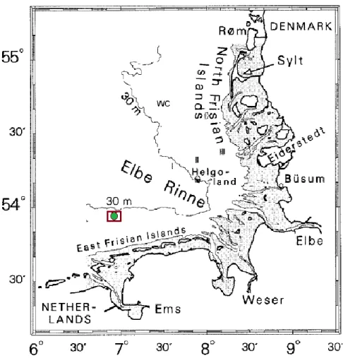
Fig. 10. Deployment point location of the ADCP data measurements.
The images of velocity direction (Fig.3) and velocity magnitude (Fig.4) represented in this Master thesis are based on the ADCP data, which was obtained during the HE-417 expedition in the German Bight from the 13th of March until 18th of March in 2014 year organized by “Marum” research center. The deployment point of the ADCP data
20
observations was located nearby the Ems river mouth, and its coordinates are 53° 59 ̍ 28 ̍ ̍ N 6° 52 ̍ 43 ̍ ̍ E, represented by the green dot in the Fig. 10.
The data of the velocity direction (Fig.3) and velocity magnitude (Fig.4) was obtained for three tidal cycles. The first tidal cycle is performed only by ebb while the flood data is absent. The second tidal cycle has data of flood and ebb and the third one has only flood data. The depth is displayed in the vertical axis and time series in the horizontal axis. The velocity direction (Fig.3) rotates from 90° during flood to - 90° during ebb.
It is possible to observe that the velocity direction for the ranges of 0 to -12 meters depth and of -12 to -30 meters depth, is different at slack water time in every tidal cycle. During the transition from ebb to flood at 13:00 and 23:00 of 13.03.2014, the velocity has rotated 30° in the upper section (0 to -12 meters) and -180° in the section from -12 meters to the bottom. Another important fact observed is the difference in the velocity direction at slack water time (19:00) for the 13.03.2014 during the transition from flood to ebb. In this case, velocity direction is -180° in the upper section of the water column (0 to -12 meters) and ranges from 40° to - 40° for the lower section (from -12 meters to the bottom).
Velocity magnitude data (Fig. 4) is obtained for three tidal cycles, however, the first tidal cycle only contains data for the ebb event (13:00 to 16:00) during the 13.03.2014. The second cycle, contains data for both events, flood and ebb (16:00 to 22:00) in the 13.03.2014. Finally, the third cycle only contains data for the flood event (22:00 to 01:00) during the 14.03.2014. Velocity magnitude varies from 0 to 0.9 m s-1 during the tidal cycle. However, tidal asymmetry in velocity magnitude is observed between flood and ebb, as a result, the values of velocity magnitude are different during flood and ebb.
Moreover, during ebb time (13:00 to 16:00) velocity magnitude increases upward from 0 m s-1 near the bottom to 0.5 m s-1. In the next tidal cycle during flood (16:00 to 19:00), velocity magnitude increases from 0 m s-1 near the bottom to 0.8 m s-1 in the range from -5 to -17 meters depth and reaches its maximum value 0.9 m s-1, near the surface. During the ebb of this tidal cycle (19:00 to 22:00), values of velocity magnitude become smaller than during flood and varies from 0 m s-1 near the bottom to 0.7 m s-1 at the top. As a final point, during the last tidal cycle, at time of flood (22:00 to 01:00), velocity magnitude increases and has a maximum value of 0.8 m s-1 in the upper part of the water column.
21
Chapter 2
Results
3.1 Idealized one-dimensional GOTM model simulations
According to the upward looking ADCP data (Fig.3 and 4), GOTM simulations are carried out to predict relevant processes and the drivers that leads to their appearance in the water column of the German Bight. For example, tidal straining and counter rotation of tidal velocity at slack water time. In addition, with the GOTM simulations, thresholds of the density salinity gradient magnitude that produces tidal straining, can be observed.
However, the tidal straining not only depends on a threshold value of the density salinity gradient magnitude, but its appearance can be defined under a ratio between the tidal velocity, the salinity gradient magnitude (which interact between each other and can vary in time) and depth of the water column. This relationship is known as the Simpson number (Simpson et al., 1990), which is responsible for governing the tidal straining dynamics (Becherer J. et al., 2011).
On the other hand, another major factor affecting the tidal straining and the counter rotation is the relative direction of the density salinity gradient, therefore, different angles of the incoming density salinity gradient must be considered in the GOTM simulations of this Master thesis.
Furthermore, the values of the tidal current velocity has the possibility to be changed during a short time period, as a result, a sensitivity analysis of this parameter would be positive for the understanding of the dynamics of the water column in the German Bight.
Therefore, it is necessary to consider several values of tidal current velocity in the settings of the GOTM model.
Following the previous order of ideas, the first step into the development of this research, is to determine the relative density salinity gradient direction as well as its magnitude.
The next step will be then, to complete the sensitivity analysis of tidal current velocity.
Thus, it is possible to determine different values of the Simpson number in order to establish a range to differentiate between the diverse dynamic regimes of the tidal flow (well mixed flow, alternation between stratified and SIPS).
22 3.2 Density salinity gradient magnitude
In order to calculate the magnitude of the density salinity gradient, the BSH observation maps of salinity were used, following the equation (7). Where 𝑆1 is 26 psu, taken as the salinity in the coastal waters area (53° 30' 00'' N and longitude 6° 52' 43'' E), near the Ems river mouth (fig. ) and 𝑆2, represents the salinity value of the deployment point where the ADCP data was obtain (53° 59' 28'' N and longitude 6° 52' 43'' E) and is equal to 33 psu.
Finally, the parameter d denotes the distance between these two areas, which are separated approximately by 30 minutes of longitude. In this case, one degree of longitude is 67138 m at 53° 30' 00'' N latitude. Therefore, the distance between 𝑆1 and 𝑆2 is 33569 m. As a result, the estimated magnitude of the density salinity gradient in the study area is -2,085
× 10-4 psu m-1.
𝜕𝑥𝑆 = 𝑆1−𝑆𝑑 2 (7) 3.3 Relative direction effect of the density salinity gradient
The following specifications were chosen as close to the real conditions where the ADCP data was obtained: water depth is kept to a constant mean value of H = 30 m, bed roughnessh0b = 0.05 m (muddy bed), tidal current mean velocity u = 0.5 m s-1, averaged between 0.3 and 0.8 m s-1 (van Alphen et al. 1988), and considered in along east-west direction. A tidal period is fixed to reproduce the semidiurnal M2 tide, with T = 44 714 s and a horizontal density salinity gradient 𝜕𝑥𝑆 = -2,085 × 10-4 psu m-1, calculated before.
Various stationary wind-forcing situations are not considered due to the absence of meaningful wind conditions during the ADCP data measurements. Salinity is relaxed to 33 psu, with a relaxation constant equal to the tidal period. Coriolis force is considered to latitude 53° 59' 28'' N. The simulations are carried out from some initial conditions such as zero velocity, minimum turbulence, constant salinity, and is settled for 10 tidal periods.
The length of the entire tidal cycle is 12.5 hours, where the flood period starts from 0 hour to 6.25 hour, while the ebb period starts from 6.25 hour and finishes at 12.5 hour. Results are shown only for the last tidal period and an interval variation of the salinity gradient direction every 45° from 0° to 360°.
In addition to the velocity direction and velocity magnitude values, the results of salinity and absolute shear were also obtained.
23
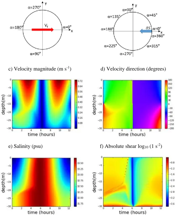
3.3.1 Relative direction of the density salinity gradient α = 0°
a) Forcing velocity direction b) Density salinity gradient direction
c) Velocity magnitude (m s-1) d) Velocity direction (degrees)
e) Salinity (psu) f) Absolute shear log10 (1 s-2)
Fig. 11. a) Tidal forcing velocity direction; b) Density salinity gradient direction;
c) Velocity magnitude (m s-1); d) Velocity direction (degrees); e) Salinity (psu);
f) Absolute shear log10 (m s-1). All graphs are shown respect to time of harmonic tide with the density salinity gradient direction from the east (α = 0°) and location 53° 59' 28'' N 6° 52' 43'' E.
24
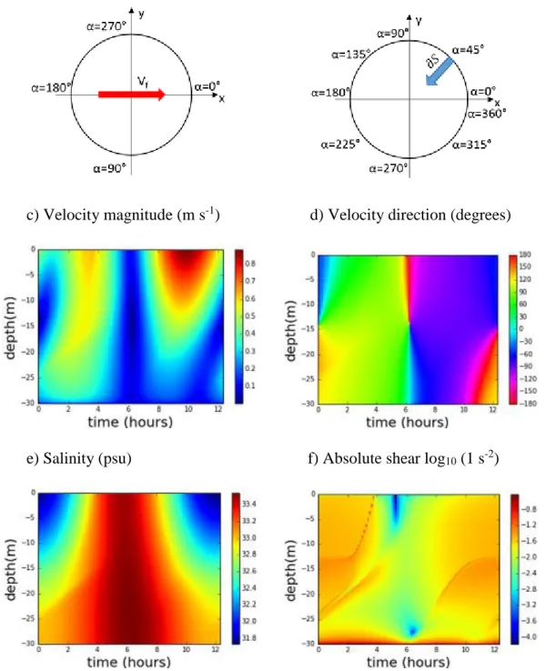
3.3.2 Relative direction of the density salinity gradient α = 45°
a) Forcing velocity direction b) Density salinity gradient direction
c) Velocity magnitude (m s-1) d) Velocity direction (degrees)
e) Salinity (psu) f) Absolute shear log10 (1 s-2)
Figure 12. a) Tidal forcing velocity; b) Density salinity gradient direction; c) Velocity magnitude (m s-1); d) Velocity direction (degrees); e) Salinity (psu); f) Absolute shear log10 (m s-1). All graphs are shown respect to time of harmonic tide with the density
salinity gradient direction from the north-east (α = 45°) and location 53° 59' 28'' N 6° 52' 43'' E.
25
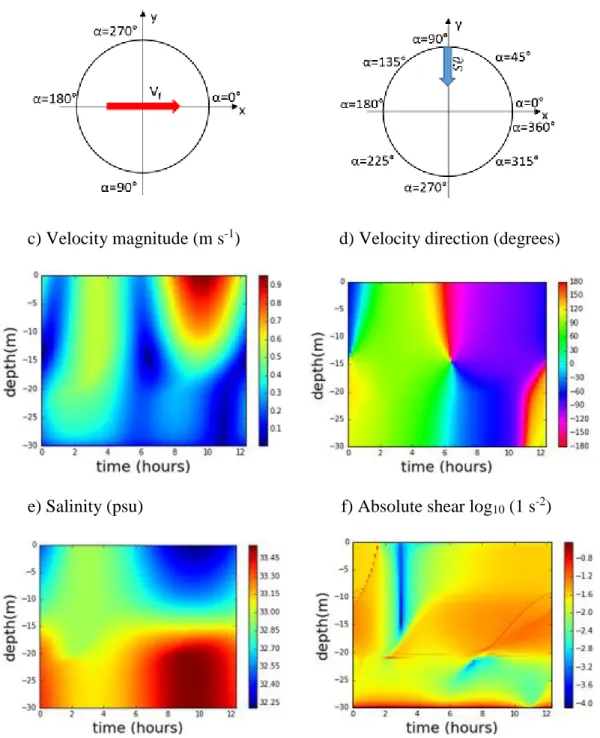
3.3.3 Relative direction of the density salinity gradient α = 90°
a) Forcing velocity direction b) Density salinity gradient direction
c) Velocity magnitude (m s-1) d) Velocity direction (degrees)
e) Salinity (psu) f) Absolute shear log10 (1 s-2)
Figure 13. a) Tidal forcing velocity; b) Density salinity gradient direction; c) Velocity magnitude (m s-1); d) Velocity direction (degrees); e) Salinity (psu); f) Absolute shear log10 (m s-1). All graphs are shown respect to time of harmonic tide with the density
salinity gradient direction from the north (α = 90°) and location 53° 59' 28'' N 6° 52' 43'' E.
26
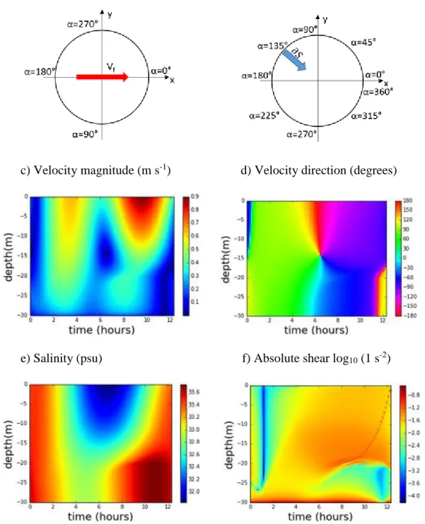
3.3.4 Relative direction of the density salinity gradient α = 135°
a) Forcing velocity direction b) Density salinity gradient direction
c) Velocity magnitude (m s-1) d) Velocity direction (degrees)
e) Salinity (psu) f) Absolute shear log10 (1 s-2)
Figure 14. a) Tidal forcing velocity; b) Density salinity gradient direction; c) Velocity magnitude (m s-1); d) Velocity direction (degrees); e) Salinity (psu); f) Absolute shear log10 (m s-1). All graphs are shown respect to time of harmonic tide with the density
salinity gradient direction from the north-west (α = 135°) and location 53° 59' 28'' N 6° 52' 43'' E.
27
3.3.5 Relative direction of the density salinity gradient α = 180°
a) Forcing velocity direction b) Density salinity gradient direction
c) Velocity magnitude (m s-1) d) Velocity direction (degrees)
e) Salinity (psu) f) Absolute shear log10 (1 s-2)
Figure 15. a) Tidal forcing velocity; b) Density salinity gradient direction; c) Velocity magnitude (m s-1); d) Velocity direction (degrees); e) Salinity (psu); f) Absolute shear log10 (m s-1). All graphs are shown respect to time of harmonic tide with the density
salinity gradient direction from the west (α = 180°) and location 53° 59' 28'' N 6° 52' 43'' E.
28
3.3.6 Relative direction of the density salinity gradient α = 225°
a) Forcing velocity direction b) Density salinity gradient direction
c) Velocity magnitude (m s-1) d) Velocity direction (degrees)
e) Salinity (psu) f) Absolute shear log10 (1 s-2)
Figure 16. a) Tidal forcing velocity; b) Density salinity gradient direction; c) Velocity magnitude (m s-1); d) Velocity direction (degrees); e) Salinity (psu); f) Absolute shear log10 (m s-1). All graphs are shown respect to time of harmonic tide with the density
salinity gradient direction from the south-west (α = 225°) and location 53° 59' 28'' N 6° 52' 43'' E.
29
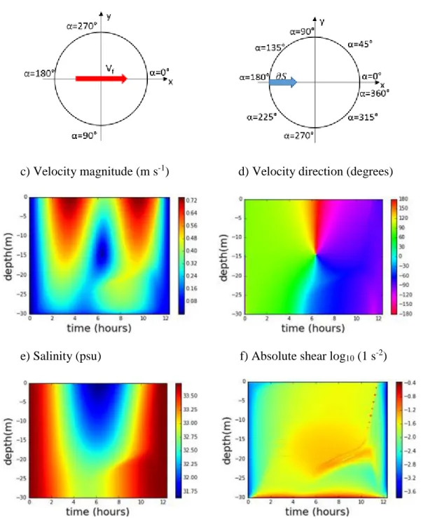
3.3.7 Relative direction of the density salinity gradient α = 270°
a) Forcing velocity direction b) Density salinity gradient direction
c) Velocity magnitude (m s-1) d) Velocity direction (degrees)
e) Salinity (psu) f) Absolute shear log10 (1 s-2)
Figure 17. a) Tidal forcing velocity; b) Density salinity gradient direction; c) Velocity magnitude (m s-1); d) Velocity direction (degrees); e) Salinity (psu); f) Absolute shear log10 (m s-1). All graphs are shown respect to time of harmonic tide with the density
salinity gradient direction from the south (α = 270°) and location 53° 59' 28'' N 6° 52' 43'' E.
30
3.3.8 Relative direction of the density salinity gradient α = 315°
a) Forcing velocity direction b) Density salinity gradient direction
c) Velocity magnitude (m s-1) d) Velocity direction (degrees)
e) Salinity (psu) f) Absolute shear log10 (1 s-2)
Figure 18. a) Tidal forcing velocity; b) Density salinity gradient direction; c) Velocity magnitude (m s-1); d) Velocity direction (degrees); e) Salinity (psu); f) Absolute shear log10 (m s-1). All graphs are shown respect to time of harmonic tide with the density
salinity gradient direction from the south-east (α = 315°) and location 53° 59' 28'' N 6° 52' 43'' E.
31
In every simulation presented before, the only parameter that varied was the direction of the density salinity gradient. These experiments were carried out in order to obtain the relative salinity gradient direction that can replicate the real values acquired with the ADCP data. The figures (a) represents the direction of the tidal current velocity, figures (b) shows the direction of the density salinity gradient (variable), figures (c) are the velocity magnitude, (d) represents the velocity direction, (e) salinity and (f) the absolute shear.
In the GOTM simulations, the tidal current flows from the west to the east and interacts with the density salinity gradient, which can be directed from different sides. For the cases when the density salinity gradient direction is α = 0° and α = 180°, these both parameters are aligned. In addition, the velocity magnitude has similar values during flood and ebb periods, showing a general decrease from 0.72 m s-1 near the surface, to 0 m s-1 near the bottom.
On the other hand, it is possible to observe tidal asymmetry between flood and ebb in the velocity magnitude for the cases when the density salinity gradient is not aligned to the tidal current velocity (Fig. 12c, 13c, 14c, 16c, 17c, 18c). When the density salinity gradient flows from the north towards the tidal current (Fig. 12c, 13c, 14c), the velocity magnitude is bigger during ebb than during flood, reaching 0.9 m s-1 near the surface at ebb times and decreasing to 0 m s-1 in the bottom. While during flood, the maximum velocity is 0.5 m s-1 near the surface, and drops to 0 m s-1 towards the bottom. If the density salinity gradient runs from the southern sides (Fig. 16c, 17c, 18c), then the opposite situation is observed. As a result, the velocity magnitude is bigger at flood times than at ebb, having the same maximum and minimum values (0.9 m s-1 for flood and 0.5 m s-1 for ebb)
The distribution of salinity in the water column (Fig. 11e, 12e, 13e, 14e, 15e, 16e, 17e and 18e) changes according to the density salinity gradient direction. The dynamic regime characterized as an alternation between stratified and well-mixed stages (strain‐induced periodic stratification ‐ SIPS), is observed only in simulations where the density salinity gradient is perpendicular to the tidal current direction, for α = 90° and α = 270° (Fig. 13e and 17e, subsequently). When the density salinity gradient direction is 90°, during the ebb period is observed a maximum value of salinity equal to 33.45 psu in the lower part of the water column (at depths from 20 to 30 meters) and a minimum value equal to 32.25 psu is located near the surface. In contrast, for the case when the density salinity gradient
32
direction is 270°, these maximum and minimum values are observed during the flood period instead of ebb period.
On the other hand, permanent stratification is observed in the water column for the cases when the density salinity gradient is not directed perpendicular to the tidal current velocity. However, permanent stratification appears in the beginning of flood and in the end of ebb, when the density salinity gradient is directed from the east sides, for α = 0°, α = 45° and α = 315° (Fig. 11e, 12e and 18e, subsequently). In these cases, salinity has maximum values at slack water time, between 33.4 and 33.8 psu at depths from 20 to 30 meters, while the minimum values oscillates around 31.75 and 32.0 psu near the surface, in the beginning of flood and in the end of ebb. Nevertheless, when the density salinity gradient is directed from the west sides, for α = 135°, 180° and 225°, (Fig. 14e, 15e and 16e) then the permanent stratification is induced mostly at slack water time. In these cases, salinity has maximum values in the beginning of flood and in the end of ebb, around 33.6 psu at depths from 20 to 30 meters, while the minimum values oscillates around 31.8 psu near the surface, at slack water time.
Velocity direction (Fig. d) changes from 90° during flood to - 90° during ebb. However, during the same periods, there are different directions of velocity observed in the water column, which can occur in the beginning of tide, at slack water time and in the end of tide. This phenomenon occurs in the beginning of tide for most of the simulations, where it is possible to observe different velocity directions between the upper and lower part of the water column during the same time. For the cases where the density salinity gradient comes from the northern sides (Fig. 12d, 13d and 14d), there is counterclockwise rotation in the upper part of the water column (depths from 0 to 15m), while clockwise rotation is observed in the lower part of the water column (from 15 to 30m depth). In contrast, when the density salinity gradient is directed from the southern sides (Fig. 16d, 17d and 18d), the velocity has a clockwise direction but it differs between upper and lower part of the water column. From 0 to 15m water depth, the velocity direction ranges from 20° up to 70°, while in the rest of the water column (15-30m), ranges from 150° up to 180°. As well as the velocity direction, absolute shear values differs in the upper and lower part of the water column during the same periods of time.
When the density salinity gradient flows from the east towards the tidal current (α = 0°), velocity direction (Fig. 11d) is 0° in the upper part of the water column, and is 150° in
the lower part. Finally, for the case when the density salinity gradient direction is α = 180° (Fig. 15d), the rotation is homogenous and equal to 90° in the entire water
33
column by the beginning of tide, where the absolute shear is also homogeneous for the same period of time (Fig. 15f).
During slack water times, it is possible to observe decoupling of the water column by different velocity directions in all simulations (Fig. 12d, 13d, 14d, 15d, 16d, 17d and 18d)
except in the one where the density salinity gradient direction moves from the east, α = 0° (Fig. 11d). The water column decoupling is represented by different velocity
rotations between upper and lower part. Velocity direction transfers from 120° to -120°
in the upper part of the water column (at depths from 0 to 15 m) and from 30° to -30° in the lower part of the water column (at depths from 15 to 30 m). In addition, strong absolute shear (around -0.8 s-2) is observed at slack water time, where decoupling of the water column by different velocity directions exist (Fig. 12f, 13f, 14f, 15f, 16f, 17f and 18f). In contrast, the absolute shear is weaker (around -3.6 s-2) at slack water time, where is no decoupling of the water column by different velocity directions (Fig. 11f).
By the end of the tidal period, when the density salinity gradient moves from northern sides (Fig. 12d, 13d and 14d), there is a clockwise rotation of 120° in the lower part of the water column (from 15 to 30 m depth) but counterclockwise rotation of -90° in the upper part of the water column (from 0 to 15 m depth). On the other hand, when the density salinity gradient is directed from the southern sides (Fig. 16d, 17d and 18d), the velocity has a counterclockwise direction along the entire water column. Nevertheless, in the upper part of the water column it is established as -90° (from 0 to 15 m depth) and in the lower part (from 15 to 30 m depth), as -120°. Moreover, the absolute shear values also differs in the upper and lower part of the water column during the same periods.
Finally, after studying the relative direction effect of the density salinity gradient, and launching the GOTM simulations (with an interval variation every 45° from 0° to 360°), the results that best reproduces the real measurements of velocity magnitude and velocity direction from the ADCP data are when the density salinity gradient has the following directions: 225° (south-west), 270° (south) and 315° (south-east).
34
3.4 Sensitivity analysis of the density salinity gradient magnitude effect
After obtaining the relative density salinity gradient direction, a sensitivity analysis of its magnitude is essential in order to determine its influence on the velocity direction and dynamic regime of the water column. The following forecast is made with the aim to determine the closest values of the density salinity gradient magnitude that could exist during the time of the ADCP data measurements. In addition, with this sensitivity analysis, it is possible to determine when the SIPS and counter rotation are vanished in the water column.
The following specifications were chosen as close to the real conditions where the ADCP data was obtained: water depth is kept to a constant mean value of H = 30 m and bed roughnessh0b = 0.05 m (muddy bed). A tidal period is fixed to reproduce the semidiurnal M2 tide, with T = 44714 s. The density salinity gradient magnitude 𝜕𝑥𝑆 is changed for each simulation from -2.4 × 10⁻⁴ psu m-1 to -0.4 × 10⁻⁴ psu m-1 every 0.4 × 10⁻⁴ psu m-1, while tidal current mean velocity is u = 0.5 m s-1.
35
3.4.1 Velocity direction response to the density salinity gradient moving from the south-west (α = 225°)
a) Strength of density salinity gradient b) Strength of density salinity gradient -2.4 × 10⁻⁴ psu m-1 -2.0 × 10⁻⁴ psu m-1
c) Strength of density salinity gradient d) Strength of density salinity gradient -1.6 × 10⁻⁴ psu m-1 -1.2 × 10⁻⁴ psu m-1
e) Strength of density salinity gradient f) Strength of density salinity gradient -0.8 × 10⁻⁴ psu m-1 -0.4 × 10⁻⁴ psu m-1
Fig. 19. Velocity direction (°) for: a) Density salinity gradient 𝜕𝑥𝑆= -2.4 × 10⁻⁴ psu m-1; b) 𝜕𝑥𝑆= -2.0 × 10⁻⁴ psu m-1; c) 𝜕𝑥𝑆= -1.6 × 10⁻⁴ psu m-1; d) 𝜕𝑥𝑆= -1.2 × 10⁻⁴ psu m-1; e) 𝜕𝑥𝑆= -0.8 × 10⁻⁴ psu m-1 and f) 𝜕𝑥𝑆= -0.4 × 10⁻⁴ psu m-1
36
3.4.2 Velocity direction response to the density salinity gradient moving from the south (α = 270°)
a) Strength of density salinity gradient b) Strength of density salinity gradient -2.4 × 10⁻⁴ psu m-1 -2.0 × 10⁻⁴ psu m-1
c) Strength of density salinity gradient d) Strength of density salinity gradient -1.6 × 10⁻⁴ psu m-1 -1.2 × 10⁻⁴ psu m-1
e) Strength of density salinity gradient f) Strength of density salinity gradient -0.8 × 10⁻⁴ psu m-1 -0.4 × 10⁻⁴ psu m-1
Fig. 20. Velocity direction (°) for: a) Density salinity gradient 𝜕𝑥𝑆= -2.4 × 10⁻⁴ psu m-1; b) 𝜕𝑥𝑆= -2.0 × 10⁻⁴ psu m-1; c) 𝜕𝑥𝑆= -1.6 × 10⁻⁴ psu m-1; d) 𝜕𝑥𝑆= -1.2 × 10⁻⁴ psu m-1; e) 𝜕𝑥𝑆= -0.8 × 10⁻⁴ psu m-1 and f) 𝜕𝑥𝑆= -0.4 × 10⁻⁴ psu m-1
37
3.4.3 Velocity direction response to the density salinity gradient moving from the south-east (α = 315°)
a) Strength of density salinity gradient b) Strength of density salinity gradient -2.4 × 10⁻⁴ psu m-1 -2.0 × 10⁻⁴ psu m-1
c) Strength of density salinity gradient d) Strength of density salinity gradient -1.6 × 10⁻⁴ psu m-1 -1.2 × 10⁻⁴ psu m-1
e) Strength of density salinity gradient f) Strength of density salinity gradient -0.8 × 10⁻⁴ psu m-1 -0.4 × 10⁻⁴ psu m-1
Fig. 21. Velocity direction (°) for: a) Density salinity gradient 𝜕𝑥𝑆= -2.4 × 10⁻⁴ psu m-1; b) 𝜕𝑥𝑆= -2.0 × 10⁻⁴ psu m-1; c) 𝜕𝑥𝑆= -1.6 × 10⁻⁴ psu m-1; d) 𝜕𝑥𝑆= -1.2 × 10⁻⁴ psu m-1; e) 𝜕𝑥𝑆= -0.8 × 10⁻⁴ psu m-1 and f) 𝜕𝑥𝑆= -0.4 × 10⁻⁴ psu m-1
38
The results presented before in Fig. 19, 20 and 21 shows that bigger changes in velocity rotations in the water column during the entire tidal cycle, are observed when the strength of the density salinity gradient is increased. For instance, it is possible to observe velocity directions of 90° in the upper part of the water column and of 150° in the lower part of the water column during the first two hours of tide, when the density salinity gradient strength is equal or bigger than -2.0 × 10⁻⁴ psu m-1 (Fig. a and b). In addition, different velocity rotations as -90° in the upper part and -150° in the lower part of the water column, exists in the end of the tidal cycle.
Moreover, counter rotation appears at slack water time, from the 5th to the 7th hour (between flood and ebb). In this case, velocity rotation is 150° in the upper part of the water column and -50° towards the bottom (Fig. 19a, 19b, 19c and 20a, 20b, 20c).
However, counter rotation starts to vanish when the density salinity gradient strength is equal or smaller than -1.2 × 10⁻⁴ psu m-1 (Fig. 19d and 20d). Furthermore, the same behavior is observed for the simulations when the density salinity gradient is directed from the south-east (α = 315°) in Fig. 21. Despite this fact, velocity direction of 150°
distributes until 20 meters depths at slack water time, while it reaches up to 15 meters
depth when the density salinity gradient is directed from the south-west, α = 225°
(Fig. 19) and the south, α = 270° (Fig. 20).
As a result of these velocity direction simulations under the influence of different strengths of the density salinity gradient, the most similar plots of velocity direction to
the ADCP data measurements were obtained when the density salinity gradient is -2.0× 10⁻⁴ psu m-1 directed from the south-west, α = 225° (Fig. 19b) and -1.6× 10⁻⁴ psu m-1 directed from the south, α = 270° (Fig. 20c). Other physical properties of the
water column such as velocity magnitude, absolute shear and salinity, were obtained in this sensitivity analysis of the effect of different density salinity gradient strengths, nevertheless, they will be compared to the ADCP data in the discussion.
39
3.4.4 Salinity response to the density salinity gradient moving from the south-west (α = 225°)
a) Strength of density salinity gradient b) Strength of density salinity gradient -2.4 × 10⁻⁴ psu m-1 -2.0 × 10⁻⁴ psu m-1
c) Strength of density salinity gradient d) Strength of density salinity gradient -1.6 × 10⁻⁴ psu m-1 -1.2 × 10⁻⁴ psu m-1
e) Strength of density salinity gradient f) Strength of density salinity gradient -0.8 × 10⁻⁴ psu m-1 -0.4 × 10⁻⁴ psu m-1
Fig. 22. Salinity (psu) for: a) Density salinity gradient 𝜕𝑥𝑆= -2.4 × 10⁻⁴ psu m-1;
b) 𝜕𝑥𝑆= -2.0 × 10⁻⁴ psu m-1; c) 𝜕𝑥𝑆= -1.6 × 10⁻⁴ psu m-1; d) 𝜕𝑥𝑆= -1.2 × 10⁻⁴ psu m-1; e) 𝜕𝑥𝑆= -0.8 × 10⁻⁴ psu m-1 and f) 𝜕𝑥𝑆= -0.4 × 10⁻⁴ psu m-1