The 29th International Conference on Probabilistic, Combinatorial and Asymptotic Methods for the Analysis of Algorithms (AofA 2018) was held in Uppsala, Sweden in June. Philippe is best known for fundamental advances in mathematical methods for the analysis of algorithms.
We Ever Need to Invent
Olle Häggström
1 Introduction
Such risks are discussed in Chapter 5, aided mainly by the Omohundro-Bostrom theory for instrumental versus ultimate AI goals, which is explained in some detail. Ideas on how to achieve a more favorable outcome are briefly discussed in Chapter 6, and some concluding remarks are provided in Chapter 7.
2 The possibility in principle
This is a very controversial issue where expert opinion varies widely, and while I admit that the question is open, I also maintain – as the first of my two main claims in this paper – that the emergence of superintelligence is a sufficiently plausible scenario. reliable for him. order taking seriously. We note in passing that the level of detail with which the human brain must be implemented on a digital computer to capture its intelligence remains a very open question [34].
3 When to expect superintelligence?
So even if we accept its existence, we should still be open to the possibility that the answer to the question addressed in the next paragraph – the question of when we can expect a super-intelligent machine – is 'never' is. The short answer to the question of when we can expect superintelligence is that we don't know: experts are very divided.
4 How suddenly?
This can be backed up by an analogy to the swan example: just as we stick to the "all swans are white" hypothesis until a non-white swan is encountered, we can stick to (H1) as long as no superintelligence has been produced [ 17]. I believe that this example would (or at least should) have made Popper nervous, because the idea behind his theory of falsificationism is to make science self-correcting [33], while in the case of stubbornly sticking to (H1) you want it yourself - correction (in case (H1) is wrong) is likely to materialize only the moment superintelligence emerges and and it is too late for us to avert an AI apocalypse - a scenario whose plausibility I argue for in section 5.
5 Goals of the superintelligent AI: Omohundro–Bostrom theory
In answer to the question "What will a superintelligent machine be inclined to do?", the Orthogonality Thesis itself obviously does little to narrow down the futile answer of "anything can happen." If that sounds like bad news, then perhaps a solution might be to make "make things that please your programmers" the ultimate goal of the machine.
6 AI Alignment
7 Concluding remarks
Hanson [23] provides a rich and fascinating description of the many social exotics such a discovery might lead to. 23 Robin Hanson. The Age of Em: Work, Love, and Life When Robots Rule the Earth.
Other Patterns
Some notation
We say that a permutation π ∈ S∗ is decomposable ifπ=σ∗τ for someσ, τ ∈S∗, and otherwise unsolvable; we also call a.
2 No restriction, T = ∅
3 Avoiding 132
J The limit variables Λσ in Theorem 2 can be expressed as functionals of a Brownian excursione(x), see [8]; the description is generally quite complicated, but some cases are simple.
4 Avoiding 321
5 Avoiding {132,312}
6 Avoiding {231,312}
On the other hand, we don't know how to calculate even the average EWσ in general; see [9] for calculations in various special cases. Thus, there exists exactly one block of any length `≥1, and a permutation π∈S∗(231,312) can be encoded by the set of block lengths.
7 Avoiding {231, 321}
8 Avoiding {132, 321}
9 Avoiding {231,312,321}
10 Avoiding {132,231,312}
11 Avoiding {132,231,321}
12 Avoiding {132,213,321}
A Symmetries
Simplicial Complexes
Oliver Cooley
Nicola Del Giudice
Mihyun Kang
Philipp Sprüssel
1 Introduction 1.1 Motivation
Model
We aim to define a model of random k-complexes starting from the binomial random (k+ 1)-uniform hypergraphGp=G(k;n, p) at the vertex [n]: the 0-simplices are the vertices of Gp, thek-simplices are the hyperedges of Gp, but there is more than one way to guarantee the downward closure property, to obtain a simple complex. In contrast, we will include only those simplexes necessary to ensure the downward closing property.
Main results
Note that Theorem 1.8 ii and iii give a shock time result for the process described above. A similar result was proved by Kahle and Pittel [15] for Yp, but only for the 2-dimensional case.
Related work
More generally, we prove that the dimension of the jth cohomology group with coefficients in F2 in distribution converges to a random Poisson variable.
2 Preliminaries
Cohomology terminology
Therefore, we can define the jth cohomology group of G with coefficients in F2 as a quotient group. It is easy to see that if is an aj-cycle and J is an aj-cycle such that f|J has a support of odd size, then f is not an aj-come and is therefore a bad function.
Minimal obstructions
Recall that a set J of j-primes is a j-cycle if every (j−1)-prime occurs in an even number of j-primes in J .
3 Subcritical regime 3.1 Overview
- Topological connectedness
- Finding obstructions
- Excluding obstructions and determining the hitting time
- Covering the interval
Define ¯pMj as the first birth time longer than ¯pj such that there are no copies of Mj in Gp. First, we use the second-moment argument to show that at time p−j−1, whp, there are "many" copies of Mj.
4 Critical window and supercritical regime
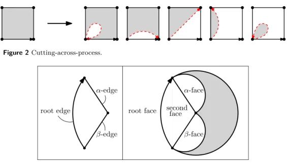
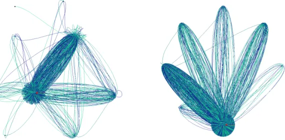
Together with the fact that whp every Mj− gives rise to a copy of Mj (Lemma 3.4), this implies that whp one copy of (K2, C2, J2) Mj exists in this interval. For the remaining interval [p−j, pMj) consider the copy (K3, C3) of Mj− which vanishes at time pMj. There exists a positive constant d¯ such that with high probability for all p≥p−j the smallest carrier of the aj-cocycle in NGp has size s To prove that pconn=pisol whp, suppose that a (k−1)-simplexσ is isolated in Ypfor someep. Then for all p≥pisol we have Yp = Gp and therefore Yp is F2-cohomologically (k−1)-connected whp for every p≥max(pisol, pMk−1) by Theorem 1.8 iii. But most|S| ≤(k−j+ 1)|I|=o(n) of these j-cycles may contain another j-simplex in S, which means that there are j-cycles meeting S only in σ, which shows that that P. 6 Concluding remarks Bret Benesh Jamylle Carter Deidra A. Coleman Douglas G. Crabill Jack H. Good Michael A. Smith Jennifer Travis 1 Overview Michael Albert Cecilia Holmgren Tony Johansson Fiona Skerman Define a partial ordering on the nodes of the tree by saying that a < bifa is an ancestor of b. This theorem gives the distribution of the number of inversions in an arbitrary split tree; where the distribution is expressed as the solution of a system of fixed point equations. Given the embedding of A0 in Tn, the number of ways to extend the embedding of H~ in Tn is at most m|A1|+|A2|. And in particular, if A0 is embedded in a |A0|-tuple not in B, there exists at most m|A1|+|A2| ways to extend to build H. The colors indicate the positions in the binary tree where the common ancestor (red), progenitor (blue) and sink (green) points are embedded. Colors indicate the positions in the split tree in which the common ancestor (red), progenitor (blue) and sink (green) points are embedded. The setGk,r is the set of acyclic digraphs that can be obtained by making copies of pathP~k and iteratively merging pairs of vertices such that each path is involved in at least one merging operation. Formally, let Gk,r be the set of directed acyclic graphs H~, so that we can find (non-disjoint) vertex subsets V1,. The second condition is to ensure that every ith path is involved in a melting operation.) For H~ ∈ Gk,r, write H~0 for H~ along with a label V1,. Andrei Asinowski Axel Bacher Cyril Banderier Since Chomsky and Schützenberger's seminal paper on the connection between context-free grammars and algebraic functions [15], which also applies to pushdown automata [30], many papers have encoded and enumerated combinatorial structures via a formal language approach. It is based on an analytical combinatorial approach, and also on the kernel method, which we used in our investigation of enumerative and asymptotic properties of. The formulas include the autocorrelation polynomial R(t, u) ofp and the small kernel root K(t, u) := (1−tP(u))R(t, u) +t`ub. The matrix kernel method leads to the formulas in Theorem 1 for the corresponding generating functions without having to solve a large algebraic system. We refer to our companion article [1] for the proofs and the complete bivariate generating functions. The dominant singularity of the generating function M(t) = (1−u1(t))Y(t)R(t,1)/K(t,1) lies on ρK =ρ and has its origin in a simple zero in the denominatorK(t, u) and fromu1. Singularity analysis thus yields the final claim of the theorem, via the following Puiseux expansion at the dominant singularityρ. These asymptotics also allow us to obtain results on limit laws, as presented in the next section. Denoting this transition by leads to formulas involving the kernel K(t, u, v) = det(I−tA) as given in equation (7), where A is the adjacency matrix of this automaton. Year after year, this claim is asserted for more and more combinatorial structures (it has been done for patterns in Markov chains, trees, maps, permutations, context-free grammars, and now.. lattice paths!). All: A Detailed History of the Future in Detail, Autobiographies of the Archangels, Faithful Library Catalogs, Thousands and Thousands of False Catalogues, Proof of the Fallacy of These Catalogues, Demonstration of the Fallacy of the True Catalogue, Basilides' Gnostic Gospel, Commentary on this Gospel, Commentary on this Gospel Commentary, The True Story of Your Death , the translation of every book into every language, the interpolation of every book in every book.” Philippe Marchal Michael Wallner The number under each node is the number of possible transitions to reach such a state. For the classical model of a single balanced Pólya urn, the limit law of the random variable Bn is fully known: The possible limit laws include a rich variety of distributions. In the next section we translate the evolution process into the language of generating functions by encoding the dynamics of this process in partial differential equations. a black ball and mex2 multiplication returning the black ball and an additional black ball into the urn. In the next section we will use equations (4) to iteratively derive the moments of the distribution of black balls after steps. In conclusion, the structure of mrin Formula (7) implies that the normalized random variable B∗n of the number of black balls in a Young-Pólya urn converges to GenGamma (1,3). The same approach allows us to study the distribution of black balls for the urn with replacement matrices M1 =M2=· · ·=Mp−1. The lower part of Figure 2 shows two trees (the "large" tree T, which contains the "small" tree S). Therefore, one can obtain a linear extension of the "large" tree T from a linear extension of the "small" tree S by a simple insertion procedure. 5 Conclusion and further work Combined with [23, Conjecture 1] and [25, Conjecture 3.3] we obtain the following explicit predictions about the diagonal coefficients. Our second set of results concerns the diagonal of the general element of the GRZ rational functionFc,d. For each suchz, if ∂Q/∂zk and detHk do not vanish, Theorem 9.2.7 of [20] identifies the integral as the corresponding summand in (14). By Borcea-Brändén's symmetrization lemma (see [7, Theorem 2.1]), the polynomial Q has no zeros in the polydisk D. This follows directly from the classical Grace-Walsh-Szegő theorem, a modern proof of which is contained in the following. Proof of Theorems 7 and 8: Suppose b is greater than the piecewise expression in the proposition; then δQ has no minimal positive zero, so the product of the three coordinates of the minimum points determined above does not lie in the positive orthans. From part (i) of Corollary 14, it suffices to check that δQ = 1−dx+cxd has a unique root of minimal modulus ρ and that ρ∈R+. We conjecture that the roots of the minimal modulus when c > c∗ are always a complex conjugate pair, however this definition does not affect our positive results. Proof of Theorem 11 InProceedings of the ACM on International Simposium on Symbolic and Algebric Computation, ISSAC ’16, bladsye 333–340, New York, NY, VSA, 2016. A Appendix A: Maple Code Maps Olivier Bodini Julien Courtiel Sergey Dovgal For the number of root edges, root degree and loops, the corresponding limit laws are normalized by n, the total number of edges. Finally, with the bijection from [10] and the known property of chord diagrams from [14], it is possible to derive limit laws for the number of leaves. Now consider the bivariate generating function X(z, v) =P. n,k>0xn,kznvk,where xn,kis is equal to the number of rooted maps with edges and vertices. The differential equation (7) is then a modification of (6) with an additional variable that marks the number of loops. Let Cn denote the number of root-ismic parts in a random rooted map with niches. LetEn denote the number of edges incident to the root vertex in a random rooted map with edges. Approximation and method of moments Another bijection in [10] is useful for proving the Poisson limit law for the number of leaves. According to [14, Theorem 2], the number of isolated edges in a random chord diagram has a Poisson distribution with parameter 1. Case of Arch Processes Matthieu Dien Antoine Genitrini In this context, one of the main goals of concurrency is to check the good behavior of such programs. Thus, the result of the method is no longer a proof of good behavior, but a statistical confirmation. The number of concurrent process runs is the number of incrementing process action flags. The following result shows a closed-form formula for the number of starts of arc processes. We note that the first terms of the series (σ(Ak+1,k))k∈N∗ coincide with the first terms of the series A220433 (shifted by 2) in OEIS2. Finally, by calculating [z1]B(z, u) with the algebraic equation it satisfies, we prove that its second derivative is a solution of the algebraic equation shown in OEISA220433. After some recursive calls, the number of xi actions has increased, and then both branches of the algorithm are taken with probabilities of the same order of magnitude. cf. As usual for unranking algorithms, the first step consists in the calculation and memory of the values of a sequence. Galton–Watson Trees Xing Shi Cai 256] have shown that the number of inversions in uniform random permutations has a central limit theorem. Note that ifT is a path, then I(T, λ) is nothing but the number of inversions in a permutation. Inversions in sequences of trees Fixed trees Random trees Similarly, define ˆΥ(Tn) as the total path length on the spheres, i.e. the sum of the depth of all balls. Then the sequence (ˆXn,Yˆn,Wˆn) defined in (1.3) converges to (ˆX,Y ,ˆ Wˆ)ind2 and in the moment generating function within the neighborhood of the origin. Conditional Galton–Watson trees Let n= (n1, . . . , nb) denote the vector of (random) numbers of balls in each of the subtrees of the root. Using the contraction method, Broutin and Holmgren [3] proved that ˆWn−→d2 is Wˆ, the unique solution of the last equation (1.4) in M10,2. For each v6=ρ also define Zv =b(Qv+ 1/2)zvc, where zv denotes the size of the subtree rooted atv. Further analysis of the moments of η and Y, including the moment generating function and tail estimates, can be found in [13]. The argument there also shows that the edge coverage time of a random-regular graph on vertices is asymptotically equal to d2((d−d−1)2)nlogn. For a non-backtracking random walk, Cooper and Frieze [7] show that the vertex and edge coverage times are asymptotically nlogn and 32nlogn, respectively. Note in particular that it shows that the expected vertex and edge coverage times are asymptotically nlogn and 32nlogn w.h.p., respectively. is. The same statement is true with the word "graphs" replaced by "configuration multigraphs" (defined in Section 3). As the process completes in time 3n/2 we see that the edge coverage time must be approx. Note that because 32n -t1 = O(δ1n), the O(logn) term only contributes an amount O(nδ1logn) =o(nlogn) to the edge coverage time. 3 Structural properties of random cubic graphs 4 Hitting times for simple random walks 5 The structure of X We bound the number of paths of length at most ω between vertices of X1 on edges of. Random walks preferring unvisited edges: Exploring high girth even degree extensions in linear time. Of course, it is interesting to consider the genus of a random graph, and such matters are also related to random graphs on surfaces (see, for example, question 8.13 of [7] and section 9 of [4]). Next, we turn to a related problem concerning the genus of a graph that is partially random. Gender is one of the most fundamental properties of a graph and plays an important role in a number of applications and algorithms (for example, color problems and the construction of electrical circuits). Consequently, our results often first involve establishing new bounds on the number of faces of G(n, m) (e.g., via the number of short cycles). We say that a property is monotonically increasing if every time an edge is added to a graph with the property, then the resulting graph also has the property. Similarly, we say that a property is monotonically decreasing if every time an edge is deleted from a graph with the property, then the resulting graph also has the property. Therefore, the number of faces of length at most i(n)ns in the giant core 2 must be . We then consider the number of faces of length at least i(n)ns in core 2 of the giant. So if we put everything together, we find that the total number of faces in the 2-core of the giant is also. We then end with an appropriate application of Euler's formula, using existing results from [12] and [13] on the number of vertices and edges in the 2-core of the giant. Let us conclude this section by noting that for lim supn→∞nk <12 the maximum degree constraint in Theorem 4 is essential, since otherwise we could take H to be a star (note that the random graph R would consist of only trees and unicyclic components and was consequently extraplanar, so that the entire graph G would then have genus zero). Matchings in Series-Parallel and Related Graph Classes The named combinatorial class is a group together with a measure of magnitude, such that ifn≥0, then the set of elements of magnitude, denoted byAn, is finite. Since there are different ways to select an item (for an element of size), the term correspondingxn/n. Finally, we will deal with the set construction of classes: given a labeled combinatorial structure A, the set construction Set(A) takes all possible sets of elements in A. If we further assume that x=ρ is the only singularity on the convergence circle|x|=ρ, which is satisfied for all our cases and for real positive constantsc0, c00, it follows (see for example [6]). Second, after each vertex of b◦j at distance one from Jj, the root of the point colored graph (L, h◦) attached to it can either be at distance one or more from L. Nevertheless, note that there exists at least one of the vertex blocks (Jj, b◦j) whose vertex is at distance one from Jj. On the assumption of strong connectedness, this radius of convergence is the same for all three solution functions C(x),D(x),E(x). If we are still within the convergence region of F, G and H, then it follows that the solution functions C(x), D(x),E(x) have a square root singularity of the form (1) atx=ρ1. Thus, a direct application of [4, Theorem 2.35] implies a central limit theorem of the proposed form, as well as the asymptotic expansions for the expected value and variance. The next step is to relate these network generating functions to the generating function B(x, y, y0, y1, y2) of independent sets in 2-connected series of parallel graphs. In the (usual) counting procedure for series-parallel graphs we have the property that ∂B∂y = x22exp(S(x, y)), where S(x, y) denotes the generating function of series networks (similar to the above) . In the latter case, the match is maximum, except for a possible pointed vertex, which may be non-matching and adjacent to other non-matching vertices. In particular, we exploit independence to ensure that the match cannot be extended. Next, note that C0 counts pointed matched graphs where the matching is maximal and the pointed vertex belongs to the independent set, C1 counts pointed matched graphs where the matching is maximal and the pointed vertex belongs to the matching, whereas C2 counts pointed matched graphs where matching is not necessarily maximal, and the pointed vertex belongs neither to the independent set nor to the matching. So, using the same arguments as just above, we see that to a vertex inIj there must be associated a vertex matched graph counted byC0, to a vertex inV(Mj) one counted byC2 and to any other vertex there must be associated a vertex matched graph counted byC1 as we need to extend the matching to maximality. Maximal matchings in series-parallel graphs The number Xn of edges with valence 3 faces on both sides in a random planar map with edges satisfies a central limit law, i.e. The background to this result is a widespread assumption that the number of pattern occurrences in planar maps (and many related graph classes) obeys a central limit theorem. To describe the DB class, we consider four different cases: both the α-face and the β-edge are equal to the root face (denoted by Dα,βB), only the α-face is equal to the root face (denoted by DαB), only the β-face is equal to the root face (denoted DβB) and neither the α-plane nor the β-plane is the same as the root plane (denoted DD) (see Fig. 4). In this case, both the α-plane and the β-plane are identical to the second plane (denoted by DψD) (see Figure 6).5 Proofs of main results 5.1 Proof of Theorem 1.8
Proof of Corollary 1.9
Proof of Theorem 1.10
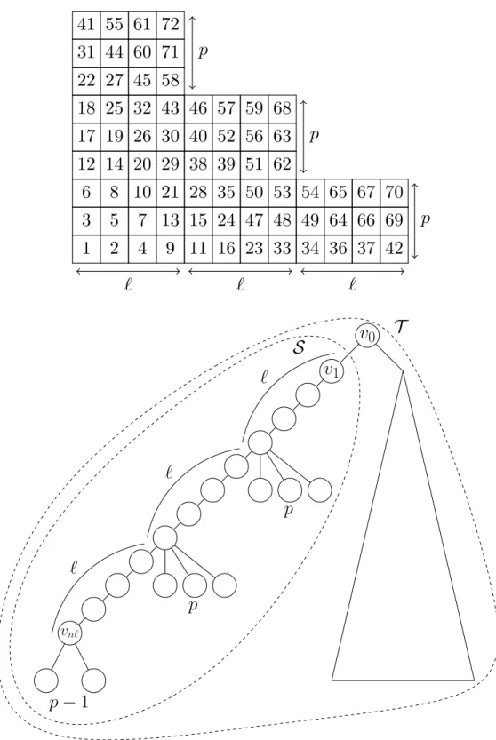
1 Introduction and statement of results
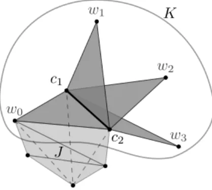
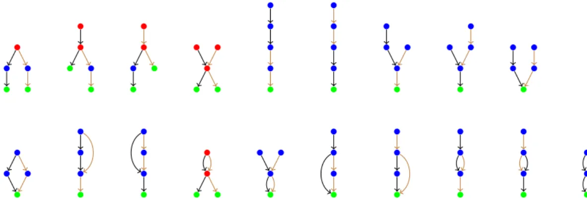
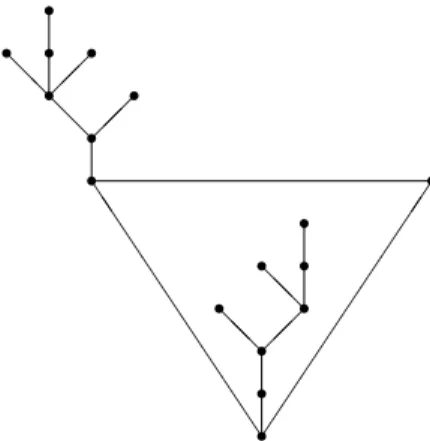
2 Embeddings of small digraphs into the complete binary tree
3 Embeddings of small digraphs into the split trees
4 Star counts
Bernhard Gittenberger
![Figure 1 Some models of self-avoiding walks are encoded by partially directed lattice paths avoiding a pattern (see [2])](https://thumb-eu.123doks.com/thumbv2/pdfplayernet/436389.50939/75.892.251.665.150.263/figure-avoiding-encoded-partially-directed-lattice-avoiding-pattern.webp)
2 Definitions and notations
3 Lattice paths with forbidden patterns and the autocorrelation polynomial
![Figure 2 The automaton for the jumps S = {−1, 1, 2} and the pattern p = [1, 2, 1, 2, −1]](https://thumb-eu.123doks.com/thumbv2/pdfplayernet/436389.50939/78.892.177.700.148.342/figure-2-automaton-jumps-s-1-1-pattern.webp)
4 Asymptotics of excursions avoiding a given pattern
5 Limit law for the number of occurrences of a given pattern
6 Conclusion
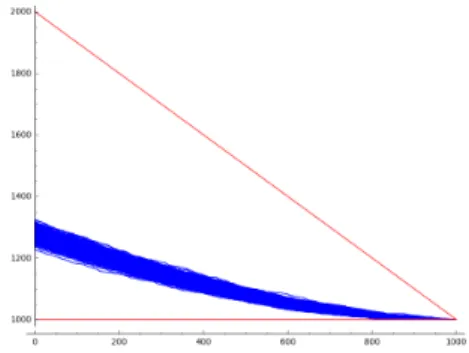
1 Periodic Pólya urns
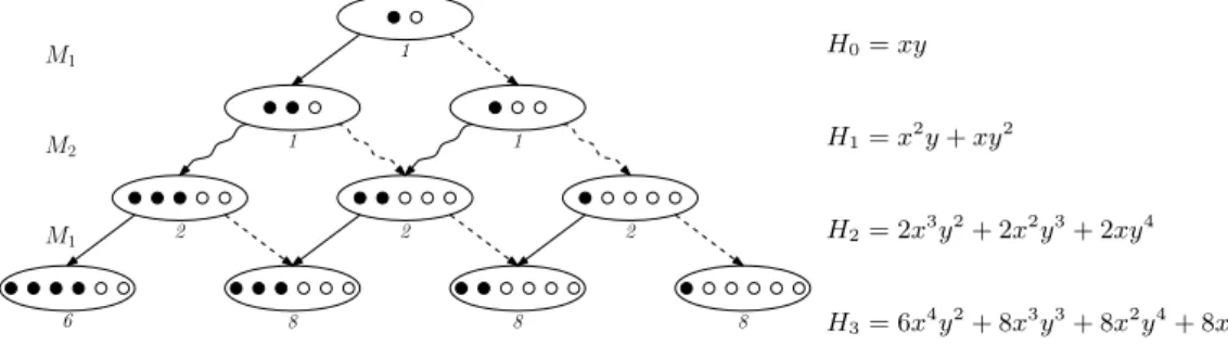
2 A functional equation for periodic Pólya urns
3 Moments of periodic Pólya urns
4 Urns, trees, and Young tableaux
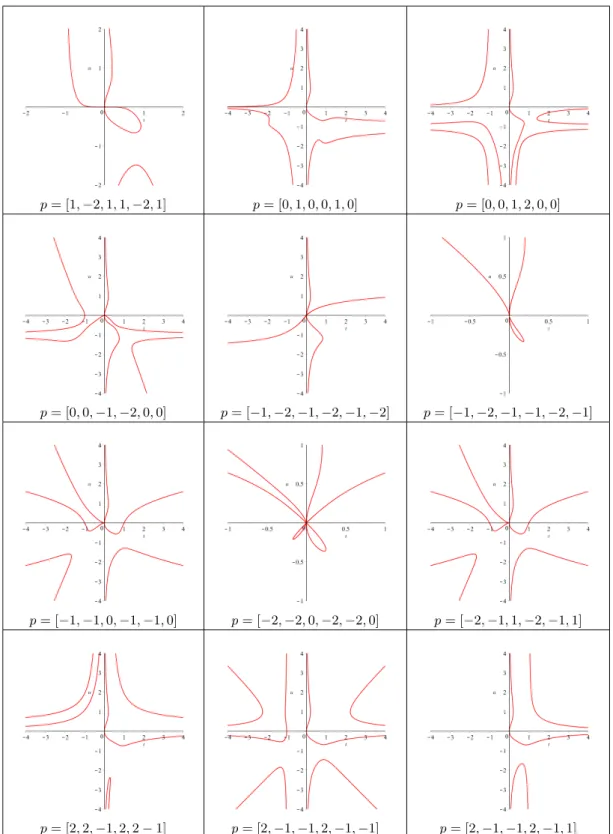
Functions via ACSV
2 ACSV
3 Symmetric multilinear functions of three variables
4 The Gillis-Reznick-Zeilberger classes
5 Lacuna computations
Hsien-Kuei Hwang
![]()
2 Differential equations for maps
3 Limit laws
Transformation into a linear differential equation
4 Combinatorics of map statistics
Alfredo Viola
2 The arch processes and their runs
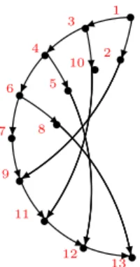
3 Algebraic generating functions
4 Uniform random generation of runs
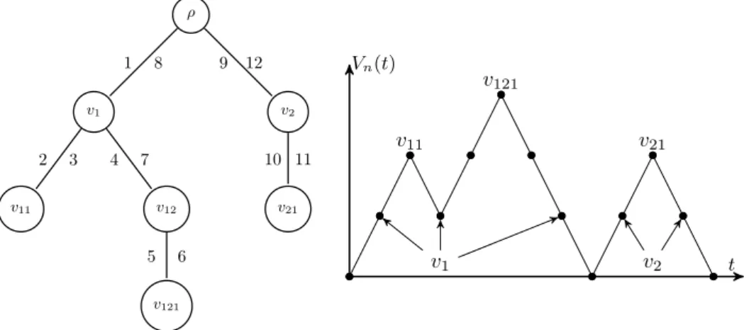
Svante Janson
Inversions in a fixed tree
Split trees
2 A sequence of split trees
Outline
3 A sequence of conditional Galton–Watson trees
Random Cubic Graph
Our results
Outlook
2 Outline proof of Theorem 2
6 Calculating the cover time 6.1 Early stages
Later Stages
Background and motivation
Main results and techniques
2 Preliminaries and notation
3 The genus of G(n,m)
4 The fragile genus property
5 Discussion
Lander Ramos
Generating functions
Graph decompositions
Asymptotics for subcritical graph classes
3 Counting in block-stable graph classes
Maximal independent sets in block-stable graph classes
Asymptotic Analysis
4 Applications
Maximal independent sets in trees
Maximal independent sets in series-parallel graphs
A Maximal matchings
Maximal matchings in block-stable classes of graphs
Maximal matchings in trees
Planar Maps
2 Combinatorics