In this study, investigation of constant and temperature-dependent thermal conductivity is implemented in receiving the temperature distribution and behavior of thermal gradient. The main goal of the master's thesis: Determination of the importance of the temperature dependence of thermal conductivity for the thermal evolution of sedimentary basins. In addition to determining how much it depends on the thermal conductivity of the rocks.
This model was used to analyze the significance of the temperature dependence of thermal conductivity for the thermal evolution of sedimentary basins in the Norwegian marginal area. In the case of temperature-dependent thermal conductivity, the model presents values closer to reality compared to constant thermal conductivity. The analysis of the results shows that the temperature-dependent thermal conductivity represents a more realistic behavior of the geothermal gradient.
Introduction
Sedimentary basins and continental margins
Scientific objectives
In this study, modeling includes investigation of temperature distribution and temperature gradient field in 1d steady-state model and parameterization of model. Source of the most important dataset of actual data on temperatures is open data from the Norwegian Petroleum Directorate (NPD). Geological data on thicknesses of sedimentary layer and crust provided from Ebbing (2010) by the Geological Survey of Norway (NGU).
Research methods include examination of available datasets (especially the Oil Directorate), examination of relevant literature on governing equations, parameters, etc. This examination includes processing of data in GIS application for creation of primary fields for distribution of parameters, processing of spatial data. Main modeling was done in the MATLAB environment (BY MathWorks), and partially in Tecmod 2D (BY GeoModelling Solutions GmbH). The main result of this study is the creation of a 1-D model for temperature gradient behavior depending on sediment and crustal thickness with the influence of constant and non-constant thermal conductivity model.
Geological settings and data
Area of investigation
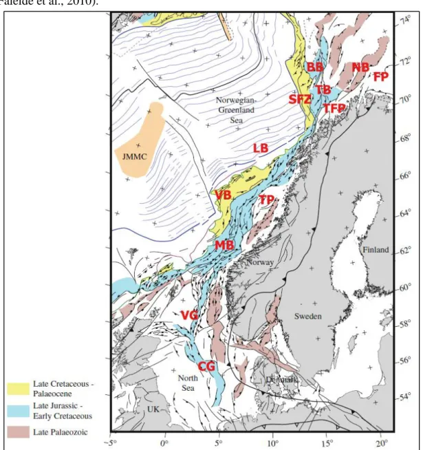
The North Sea area is not part of the Norwegian part, but is interesting as part of the Norwegian continental shelf and because of the good availability of well data. Structure of the response of the Norwegian margin to the early breakup of the Cenozoic continent and the opening of the Norwegian and Greenland Seas. Morphologically, Norwegian consists of a continental shelf and a slope that vary considerably in width and steepness.
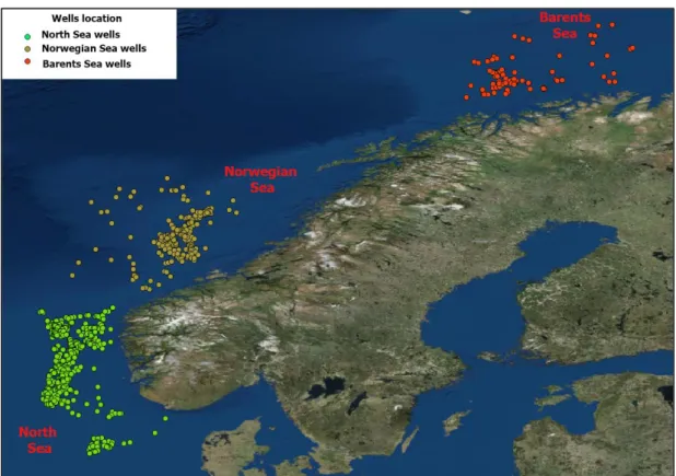
In this study, the study area is divided into three parts with similar geological and spatial conditions (Figure 1). Third research area located in the area of the northern North Sea, west - southwest of the Norwegian coast.
Geological settings
This fact results in some similarities in the stratigraphy between these areas, but some differences should be taken into account, especially during the Cretaceous and Cenozoic after the breakup and with the formation and filling of the basins (in the case of the Norwegian margin) (Faleide et al., 2008). ). The North Sea represents an example of intracratonic basins, which means that the basins lie on the continental crust (Faleide et al., 2010). The origin of the Mid-Norwegian margin is related to series of thinning and subsidence during the Cretaceous and Paleocene (Faleide et al., 2010).
Most of the structural relief was filled in by the middle of the Cretaceous (Faleide et al., 2008). The Vøring Basin has a number of sub-basins with highs, related to the Late Jurassic - Early Cretaceous (Faleide et al., 2008). In the study area, the continental margin consists of three segments: the southern shear margin along the Senja fault zone, a central rifted complex southwest of Bjørnøya associated with volcanism and a northern, originally sheared and later rifted margin along the Hornsund fault zone (Faleide et al., 2008 ).
Initial Dataset
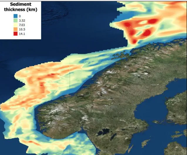
The total thickness of sediments varies from several meters (e.g. in the coastal area of the Norwegian coast, in the Trøndelag Platform) to about 15 km in basin areas (e.g. in the area of the Vøring Basin). The total thickness of sediments varies from several meters (e.g. in the area between Loppa Høje and the Bjørnøya basin) to about 15 km in basin areas (e.g. in the area of the Bjørnøya basin). However, it must be taken into account that the temperature value in the bottom holes is only measured from a point on the bottom of the well, excluding values along the wells. This fact is important because local parameters for each well may represent different properties of rock types.
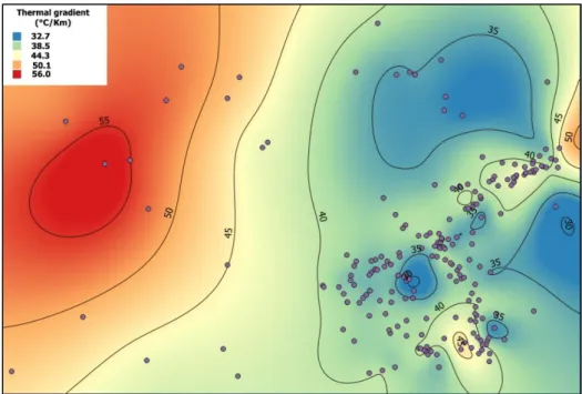
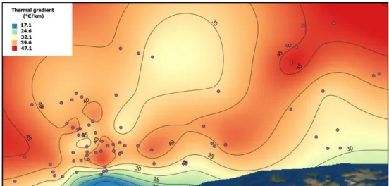
A primary temperature distribution field, a sediment and crustal thickness field in different areas of the Norwegian margin were generated in the QGIS environment. These fields allow a first conclusion about the dependence of the temperature gradient on the thickness of the sediments/crust. Based on these fields, primary figures of temperature distribution and thermal gradient behavior were generated.
Modeling approaches
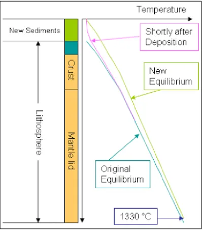
Background on sediment blanketing
Sediment has a much lower thermal conductivity compared to crustal values, implying changes in lithosphere geothermal energy (Figure 4). In the case of a constant temperature boundary condition at the base of the lithosphere, higher thermal conductivity of the sediment leads to lower temperatures in sediments and higher heat flux from the crust. In the case of a constant basement heat flow boundary condition, a lower thermal conductivity of the sediment leads to a shift of crustal and mantle values towards higher temperatures.
Consequently, the effect of sediment overlay depends on the thermal conductivity contrast between the crust and the sediments (Theissen & Rüpke, 2010; Wangen, 1995). The effects of sediment overlay not only modify the steady-state geothermal temperature, but also have a strong control on the evolution of the heat flow. However, the thermal conductivity of rocks in nature is not the same and depends on temperature and porosity.
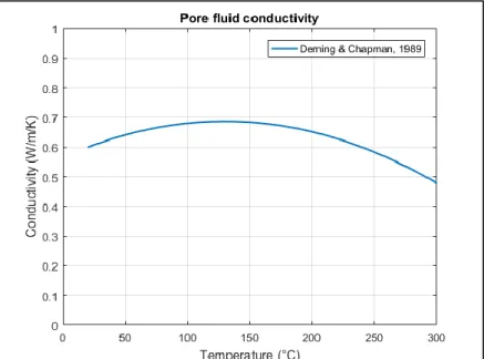
Temperature dependence of thermal conductivity
- Temperature dependence of thermal conductivity of sediments
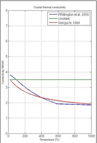
- Temperature dependence of thermal conductivity of crust
- Temperature dependence of thermal conductivity of mantle
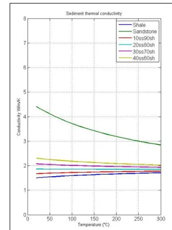
Temperature dependence of thermal conductivity in sediments for shale, sandstone and mixed lithology consisting of different fractions of sandstone and shale. Behavior of temperature dependence of thermal conductivity of sediments according to equation (2) presented in Fig. 6. Thermal conductivity for crust was calculated based on several equations referring to temperature dependence of thermal diffusion and specific heat capacity.
The temperature dependence of the thermal diffusivity for the crust can be estimated using the equations of Whittington et al. The behavior of the temperature dependence of the thermal conductivity of the crust according to the previous equations presented in Figure 8. The resulting line for thermal conductivity is represented by the behavior of the thermal conductivity according to Sekiguchi (1984) and in the case of a constant value.
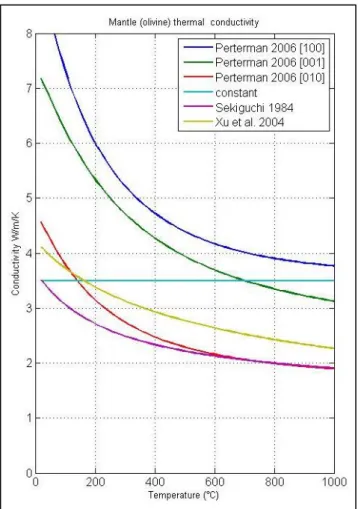
Thermal conductivity for mantle was calculated in the same way as crust, based on several equations referring to temperature dependence of thermal diffusivity and specific heat capacity. After calculations of thermal diffusivity and specific heat capacity, thermal conductivity for crust was calculated in the same way as equation (8). Behavior of temperature dependence of thermal conductivity of olivine (mantle) according to previous equations presented in figure 9.
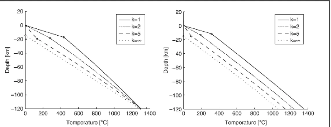
The study of the temperature dependence of the thermal conductivity was done by creating 1-D modeling at the scale of the thickness of the lithosphere. Temperature-dependence of thermal conductivity in Mantel according to different authors and in constant case. The calculation of temperatures is based on the dependence on the effective thermal conductivity of the layer material and the radiogenic heat production in each layer.
In the case of crust and mantle, scaling of the radioactive heat production by e-fold length was used (equation 14).
Results
- Temperature distribution and thermal gradient
- Crustal and sediment thicknesses
- Isostasy compensation correction
- Radiogenic heat production correction
- Thermal conductivity and thermal-gradient
- Barents Sea area
- Norwegian Sea area
- North Sea area
Modeling of thermal gradient behavior according to the introduction of governing equation and parameters in the case of constant thermal conductivity presented in figures 23-34. Figures 23-26 presented results for modeled thermal-gradient crustal and actual thermal-gradient values for Barents Sea area. In the case of value of radiogenic heat production equal to 1 x 10⁻⁶ W/𝑚3 (figure 23), we observe in modeled distribution of thermal gradient small dependence on sediment thicknesses, due to the supply of heat through sediments.
In the case of the radiogenic heat production value equal to 1 x 10⁻⁶ W/𝑚3 (figure 25), we observe the narrow situation of thermal gradient distribution. Figures 27-30 show the results for the modeled thermal gradient crust and the real thermal gradient values for the Norwegian Sea area. In case of radiogenic heat production value equal to 1 x 10⁻⁶ W/𝑚3 (figure 27), we observe the behavior of the modeled thermal gradient similar to the Barents Sea area.
The dependence of the thermal gradient on the thickness of the crust and the increase of the gradient with additional radiogenic heat production of the sediments are presented. As in the case of the Barents Sea, the model results do not match the real thermal gradient in the direction of change. The thermal gradient is mainly determined by the crustal thickness change as in the case of the Barents Sea with the same deviation of the sediment load behavior.
In the case of a value of radiogenic heat production equal to 1 x 10⁻⁶ W/𝑚3 (Figure 31), general behavior of modeled thermal gradient similar to previous regions. In the case where the production of radiogenic heat is negligible (Figures 32), the modeled thermal gradient is highly dependent on the thickness of the Earth's crust. Modeled thermal gradient range for thickness values has a lower limit and ranges from 25.
Modeled dependence of thermal gradient on crustal and sediment thickness (contour lines, step – 5°C) and real values (points) of thermal gradient for the Barents Sea area. Modeled dependence of thermal gradient on crustal and sediment thickness (contour lines, step – 5°C) and real values (points) of thermal gradient for the Norwegian Sea area. Modeled dependence of thermal gradient on crustal and sediment thickness (contour lines, step – 5°C) and real values (points) of thermal gradient for the North Sea area.
Discussion
The most interesting feature is that in the case of temperature-dependent conductivity and RHP = 1 x 10⁻⁶ W/m3, there is a range of crustal and sedimentary thicknesses as the thermal gradient decreases. According to the results, this effect occurred in an environment with a thick crust (>20 km) and a relatively small sedimentary layer (0-10 km). In real data, basins are complex in nature, represented as a combination of layers with different rock properties.
In this study, the basins were assumed to be filled with shale in the model - with appropriate properties. By changing the input of rock properties, for example in the case of limestones, thermal conductivity will increase (Hantschel, 2009). Comparing the temperature-dependent and constant thermal conductivity results, the first setting represented a more realistic range of values that could be corrected for the input rock properties.
Considering two scenarios of radiogenic heat production in sediments, there is no clear agreement with real data, but the case with RHP = zero can be considered a more realistic one. Increased production of radiogenic heat production one of the features of clay compared to other types of sediments (for example, sandstones). In addition, taking into account the fit of radiogenic heat production (presented in chapter 4.4.), the case of zero RHS presents a more realistic fit to the real data in the temperature-dependent thermal conductivity configuration.
In the case of constant thermal conductivity RHS = 1 x 10⁻⁶ W/m3 presents more valid results, however, lower geothermal than should be observed (except for the example of the North Sea area).
Conclusion
Acknowledgment
Terrestrial heat flow studies and the structure of the lithosphere A method for determining terrestrial healing flow in oil basin areas. Feedback of sedimentation on crustal heat flow: New insights from the Voring Basin, Norwegian Sea. The thermal blanketing effect of sediments on the rate and amount of subsidence in extensional sedimentary basins, Tectonophysics.
Appendix