Spiked Models in Large Random Matrices and two statistical applications
Jamal Najim [email protected]
CNRS & Universit´e Paris Est
Linstat- Link¨oping, Sweden - August 2014
1
Introduction
Large Random Matrices Objectives
Basic technical means Large covariance matrices Spiked models
Statistical Test for Single-Source Detection Direction of Arrival Estimation
Conclusion
Large covariance matrices I
The model
I Consider aN×nmatrixXN with i.i.d. entries EXij= 0, E|Xij|2= 1.
I LetRN be adeterministicN×N nonnegative definite hermitian matrix.
I Consider
YN=R1/2N XN.
MatrixYN is an-sample ofN-dimensional vectors:
YN= [Y·1 · · · Y·n] with Y·1=R1/2N X·1 and EY·1Y∗·1=RN.
I RN often calledPopulation covariance matrix.
Objective
To understand the spectrum of 1nYNY∗N as
N, n→ ∞ ⇔ N
n →c∈(0,∞)
3
Large covariance matrices I
The model
I Consider aN×nmatrixXN with i.i.d. entries EXij= 0, E|Xij|2= 1.
I LetRN be adeterministicN×N nonnegative definite hermitian matrix.
I Consider
YN=R1/2N XN. MatrixYN is an-sample ofN-dimensional vectors:
YN= [Y·1 · · · Y·n] with Y·1=R1/2N X·1 and EY·1Y∗·1=RN .
I RNoften calledPopulation covariance matrix.
Objective
To understand the spectrum of 1nYNY∗N as
N, n→ ∞ ⇔ N
n →c∈(0,∞)
3
Large covariance matrices II
Remarks
1. The asymptotic regimeN, n→ ∞and Nn →c∈(0,∞)corresponds to the case where the data dimensionis of the same orderas the number of available samples.
2. IfNfixed andn→ ∞(small data, large samples) then 1
nYNY∗N−→RN
The spectral measure of a matrix A
.. also called theempirical measure of the eigenvalues
IfAisN×N hermitian with eigenvaluesλ1,· · ·, λN then itsspectral measureis:
LN= 1 N
N
X
i=1
δλi(A) ⇒ LN([a, b]) = #{λi(A)∈[a, b]} N Otherwise stated
LN([a, b])is theproportionof eigenvalues ofAin[a, b].
Large covariance matrices II
Remarks
1. The asymptotic regimeN, n→ ∞and Nn →c∈(0,∞)corresponds to the case where the data dimensionis of the same orderas the number of available samples.
2. IfNfixed andn→ ∞(small data, large samples) then 1
nYNY∗N−→RN
The spectral measure of a matrix A
.. also called theempirical measure of the eigenvalues
IfAisN×N hermitian with eigenvaluesλ1,· · ·, λN then itsspectral measureis:
LN= 1 N
N
X
i=1
δλi(A) ⇒ LN([a, b]) = #{λi(A)∈[a, b]} N
Otherwise stated
LN([a, b])is theproportionof eigenvalues ofAin[a, b].
4
Large covariance matrices II
Remarks
1. The asymptotic regimeN, n→ ∞and Nn →c∈(0,∞)corresponds to the case where the data dimensionis of the same orderas the number of available samples.
2. IfNfixed andn→ ∞(small data, large samples) then 1
nYNY∗N−→RN
The spectral measure of a matrix A
.. also called theempirical measure of the eigenvalues
IfAisN×N hermitian with eigenvaluesλ1,· · ·, λN then itsspectral measureis:
LN= 1 N
N
X
i=1
δλi(A) ⇒ LN([a, b]) = #{λi(A)∈[a, b]} N Otherwise stated
LN([a, b])is theproportionof eigenvalues ofAin[a, b].
Large covariance matrices II
Remarks
1. The asymptotic regimeN, n→ ∞and Nn →c∈(0,∞)corresponds to the case where the data dimensionis of the same orderas the number of available samples.
2. IfNfixed andn→ ∞(small data, large samples) then 1
nYNY∗N−→RN
The spectral measure of a matrix A
.. also called theempirical measure of the eigenvalues
IfAisN×N hermitian with eigenvaluesλ1,· · ·, λN then itsspectral measureis:
LN= 1 N
N
X
i=1
δλi(A)
⇒ LN([a, b]) = #{λi(A)∈[a, b]} N
Otherwise stated
LN([a, b])is theproportionof eigenvalues ofAin[a, b].
4
Large covariance matrices II
Remarks
1. The asymptotic regimeN, n→ ∞and Nn →c∈(0,∞)corresponds to the case where the data dimensionis of the same orderas the number of available samples.
2. IfNfixed andn→ ∞(small data, large samples) then 1
nYNY∗N−→RN
The spectral measure of a matrix A
.. also called theempirical measure of the eigenvalues
IfAisN×N hermitian with eigenvaluesλ1,· · ·, λN then itsspectral measureis:
LN= 1 N
N
X
i=1
δλi(A) ⇒ LN([a, b]) = #{λi(A)∈[a, b]}
N
Otherwise stated
LN([a, b])is theproportionof eigenvalues ofAin[a, b].
4
Introduction
Large Random Matrices Objectives
Basic technical means Large covariance matrices Spiked models
Statistical Test for Single-Source Detection Direction of Arrival Estimation
Conclusion
Objectives of this talk
1. to describe the limiting spectral properties of the large covariance matrix 1
nYnYn∗=1
nR1/2n XnX∗nR1/2n
2. to study a particular class of covariance matrix models: spiked models, for which one or several eigenvalues are clearly separated from the mass of the other eigenvalues.
3. to present two applications of these results instatistical signal processing: signal detection and direction of arrival estimation.
6
Objectives of this talk
1. to describe the limiting spectral properties of the large covariance matrix 1
nYnYn∗=1
nR1/2n XnX∗nR1/2n
2. to study a particular class of covariance matrix models: spiked models, for which one or several eigenvalues are clearly separated from the mass of the other eigenvalues.
3. to present two applications of these results instatistical signal processing: signal detection and direction of arrival estimation.
6
Introduction
Large Random Matrices Objectives
Basic technical means
Large covariance matrices Spiked models
Statistical Test for Single-Source Detection Direction of Arrival Estimation
Conclusion
Spectrum and eigenvectors analysis
The resolvent
I The resolvent ofAis Q(z) = (A−zI)−1
I its singularities are exactlyeigenvaluesofA.
I Problem: if size ofAbig, then size ofQbigas well.
The normalized trace of the resolvent
I Function
gn(z) = 1
NTrace (A−zI)−1 provides information on thespectrumofA.
I It is theStieltjes transformof the spectral measure ofA(cf. supra)
8
Spectrum and eigenvectors analysis
The resolvent
I The resolvent ofAis Q(z) = (A−zI)−1
I its singularities are exactlyeigenvaluesofA.
I Problem: if size ofAbig, then size ofQbigas well.
The normalized trace of the resolvent
I Function
gn(z) = 1
NTrace (A−zI)−1 provides information on thespectrumofA.
I It is theStieltjes transformof the spectral measure ofA(cf. supra)
8
Spectrum and eigenvectors analysis
The resolvent
I The resolvent ofAis Q(z) = (A−zI)−1
I its singularities are exactlyeigenvaluesofA.
I Problem: if size ofAbig, then size ofQbigas well.
The normalized trace of the resolvent
I Function
gn(z) = 1
NTrace (A−zI)−1 provides information on thespectrumofA.
I It is theStieltjes transformof the spectral measure ofA(cf. supra)
Spectrum analysis: The Stieltjes Transform
Given a probabilityP, itsStieltjes transformis defined by g(z) =
Z
R
P(dλ)
λ−z , z∈C+,
with inverse formula Z
f dP = 1 πlim
y↓0= Z
R
f(x)g(x+iy)dx ,
forf bounded continuous.
Properties
1. Convergence in distribution is characterized by pointwise convergence of Stieltjes transforms:
Pn
−−−−→D
n→∞ P ⇔ ∀z∈C+, gn(z) =
Z Pn(dλ)
λ−z −−−−→
n→∞ g(z) =
Z P(dλ) λ−z 2. Spectral measure:
P= 1 N
N
X
i=1
δλi(A) ⇒ gn(z) = 1 N
N
X
i=1
1
λi(A)−z = 1
NTrace (A−zI)−1
The Stieltjes transfomgnis thenormalized traceof the resolvent(A−zI)−1
9
Spectrum analysis: The Stieltjes Transform
Given a probabilityP, itsStieltjes transformis defined by g(z) =
Z
R
P(dλ)
λ−z , z∈C+, with inverse formula
Z
f dP = 1 πlim
y↓0= Z
R
f(x)g(x+iy)dx ,
forf bounded continuous.
Properties
1. Convergence in distribution is characterized by pointwise convergence of Stieltjes transforms:
Pn
−−−−→D
n→∞ P ⇔ ∀z∈C+, gn(z) =
Z Pn(dλ)
λ−z −−−−→
n→∞ g(z) =
Z P(dλ) λ−z 2. Spectral measure:
P= 1 N
N
X
i=1
δλi(A) ⇒ gn(z) = 1 N
N
X
i=1
1
λi(A)−z = 1
NTrace (A−zI)−1
The Stieltjes transfomgnis thenormalized traceof the resolvent(A−zI)−1
Spectrum analysis: The Stieltjes Transform
Given a probabilityP, itsStieltjes transformis defined by g(z) =
Z
R
P(dλ)
λ−z , z∈C+, with inverse formula
Z
f dP = 1 πlim
y↓0= Z
R
f(x)g(x+iy)dx ,
forf bounded continuous.
Properties
1. Convergence in distribution is characterized by pointwise convergence of Stieltjes transforms:
Pn
−−−−→D
n→∞ P ⇔ ∀z∈C+, gn(z) =
Z Pn(dλ)
λ−z −−−−→
n→∞ g(z) =
Z P(dλ) λ−z
2. Spectral measure:
P= 1 N
N
X
i=1
δλi(A) ⇒ gn(z) = 1 N
N
X
i=1
1
λi(A)−z = 1
NTrace (A−zI)−1
The Stieltjes transfomgnis thenormalized traceof the resolvent(A−zI)−1
9
Spectrum analysis: The Stieltjes Transform
Given a probabilityP, itsStieltjes transformis defined by g(z) =
Z
R
P(dλ)
λ−z , z∈C+, with inverse formula
Z
f dP = 1 πlim
y↓0= Z
R
f(x)g(x+iy)dx ,
forf bounded continuous.
Properties
1. Convergence in distribution is characterized by pointwise convergence of Stieltjes transforms:
Pn
−−−−→D
n→∞ P ⇔ ∀z∈C+, gn(z) =
Z Pn(dλ)
λ−z −−−−→
n→∞ g(z) =
Z P(dλ) λ−z 2. Spectral measure:
P= 1 N
N
X
i=1
δλi(A) ⇒ gn(z) = 1 N
N
X
i=1
1
λi(A)−z = 1
NTrace (A−zI)−1
The Stieltjes transfomgnis thenormalized traceof the resolvent(A−zI)−1
Spectrum analysis: The Stieltjes Transform
Given a probabilityP, itsStieltjes transformis defined by g(z) =
Z
R
P(dλ)
λ−z , z∈C+, with inverse formula
Z
f dP = 1 πlim
y↓0= Z
R
f(x)g(x+iy)dx ,
forf bounded continuous.
Properties
1. Convergence in distribution is characterized by pointwise convergence of Stieltjes transforms:
Pn
−−−−→D
n→∞ P ⇔ ∀z∈C+, gn(z) =
Z Pn(dλ)
λ−z −−−−→
n→∞ g(z) =
Z P(dλ) λ−z 2. Spectral measure:
P= 1 N
N
X
i=1
δλi(A) ⇒ gn(z) = 1 N
N
X
i=1
1
λi(A)−z = 1
NTrace (A−zI)−1
The Stieltjes transfomgnis thenormalized traceof the resolvent(A−zI)−1
9
Introduction
Large covariance matrices
Wishart matrices and Marˇcenko-Pastur’s theorem The general covariance model
Spiked models
Statistical Test for Single-Source Detection Direction of Arrival Estimation
Conclusion
Wishart Matrices
The model
I We first focus on covariance matrices in the case where RN=σ2IN .
I HenceYNis aN×nmatrix with i.i.d. entriesEYij= 0, E|Yij|2=σ2.
I Matrix n1YNYN∗ is aWishart matrix.
The standard case N << n
AssumeN fixed andn→ ∞(small data, large sample). Since EY·1Y∗·1=σ2IN ,
L.L.N implies 1
nYNYN∗ = 1 n
n
X
i=1
Y·iY∗·i −−−−→a.s.
n→∞ σ2IN
In particular,
I all the eigenvalues of n1YNYN∗ converge toσ2,
I equivalently, the spectral measure of n1YNYN∗ converges toδσ2.
11
Wishart Matrices
The model
I We first focus on covariance matrices in the case where RN=σ2IN .
I HenceYNis aN×nmatrix with i.i.d. entriesEYij= 0, E|Yij|2=σ2.
I Matrix n1YNYN∗ is aWishart matrix.
The standard case N << n
AssumeN fixed andn→ ∞(small data, large sample). Since EY·1Y∗·1=σ2IN ,
L.L.N implies 1
nYNYN∗ = 1 n
n
X
i=1
Y·iY∗·i −−−−→a.s.
n→∞ σ2IN
In particular,
I all the eigenvalues of n1YNYN∗ converge toσ2,
I equivalently, the spectral measure of n1YNYN∗ converges toδσ2.
11
Wishart Matrices
The model
I We first focus on covariance matrices in the case where RN=σ2IN .
I HenceYNis aN×nmatrix with i.i.d. entriesEYij= 0, E|Yij|2=σ2.
I Matrix n1YNYN∗ is aWishart matrix.
The standard case N << n
AssumeN fixed andn→ ∞(small data, large sample).
Since EY·1Y∗·1=σ2IN ,
L.L.N implies 1
nYNYN∗ = 1 n
n
X
i=1
Y·iY∗·i −−−−→a.s.
n→∞ σ2IN
In particular,
I all the eigenvalues of n1YNYN∗ converge toσ2,
I equivalently, the spectral measure of n1YNYN∗ converges toδσ2.
Wishart Matrices
The model
I We first focus on covariance matrices in the case where RN=σ2IN .
I HenceYNis aN×nmatrix with i.i.d. entriesEYij= 0, E|Yij|2=σ2.
I Matrix n1YNYN∗ is aWishart matrix.
The standard case N << n
AssumeN fixed andn→ ∞(small data, large sample). Since EY·1Y∗·1=σ2IN,
L.L.N implies 1
nYNYN∗ = 1 n
n
X
i=1
Y·iY∗·i −−−−→a.s.
n→∞ σ2IN
In particular,
I all the eigenvalues of n1YNYN∗ converge toσ2,
I equivalently, the spectral measure of n1YNYN∗ converges toδσ2.
11
Wishart Matrices
The model
I We first focus on covariance matrices in the case where RN=σ2IN .
I HenceYNis aN×nmatrix with i.i.d. entriesEYij= 0, E|Yij|2=σ2.
I Matrix n1YNYN∗ is aWishart matrix.
The standard case N << n
AssumeN fixed andn→ ∞(small data, large sample). Since EY·1Y∗·1=σ2IN,
L.L.N implies 1
nYNYN∗ = 1 n
n
X
i=1
Y·iY∗·i −−−−→a.s.
n→∞ σ2IN
In particular,
I all the eigenvalues of n1YNYN∗ converge toσ2,
I equivalently, the spectral measure of n1YNYN∗ converges toδσ2.
11
Marˇ cenko-Pastur theorem
Theorem
I Consider thespectral measureLN:
LN= 1 N
N
X
i=1
δλi, λi=λi
1 nYNY∗N
I Thenalmost surely(= for almost every realization) LN−−−−−−→
N,n→∞ PMPˇ in distribution as N n −−−−→
n→∞ c∈(0,∞) wherePMPˇ isMarˇcenko-Pasturdistribution:
PMPˇ (dx) =
1−1 c
+
δ0(dx) +
p(b−x)(x−a)
2πσ2xc 1[a,b](x)dx
with
a = σ2(1−√ c)2 b = σ2(1 +√
c)2
12
Marˇ cenko-Pastur theorem
Theorem
I Consider thespectral measureLN:
LN= 1 N
N
X
i=1
δλi, λi=λi
1 nYNY∗N
I Thenalmost surely(= for almost every realization) LN−−−−−−→
N,n→∞ PMPˇ in distribution as N n −−−−→
n→∞ c∈(0,∞)
wherePMPˇ isMarˇcenko-Pasturdistribution:
PMPˇ (dx) =
1−1 c
+
δ0(dx) +
p(b−x)(x−a)
2πσ2xc 1[a,b](x)dx
with
a = σ2(1−√ c)2 b = σ2(1 +√
c)2
Marˇ cenko-Pastur theorem
Theorem
I Consider thespectral measureLN:
LN= 1 N
N
X
i=1
δλi, λi=λi
1 nYNY∗N
I Thenalmost surely(= for almost every realization) LN−−−−−−→
N,n→∞ PMPˇ in distribution as N n −−−−→
n→∞ c∈(0,∞) wherePMPˇ isMarˇcenko-Pasturdistribution:
PMPˇ (dx) =
1−1 c
+
δ0(dx) +
p(b−x)(x−a)
2πσ2xc 1[a,b](x)dx
with
a = σ2(1−√ c)2 b = σ2(1 +√
c)2
12
Marˇ cenko-Pastur theorem
Theorem
I Consider thespectral measureLN:
LN= 1 N
N
X
i=1
δλi, λi=λi
1 nYNY∗N
I Thenalmost surely(= for almost every realization) LN−−−−−−→
N,n→∞ PMPˇ in distribution as N n −−−−→
n→∞ c∈(0,∞) wherePMPˇ isMarˇcenko-Pasturdistribution:
PMPˇ (dx) =
1−1 c
+
δ0(dx) +
p(b−x)(x−a)
2πσ2xc 1[a,b](x)dx
with
a = σ2(1−√ c)2 b = σ2(1 +√
c)2
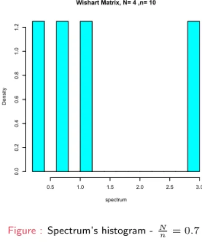
Histogram for Wishart matrices
: Marˇ cenko-Pastur’s theorem
Matrix model: Wishart matrix
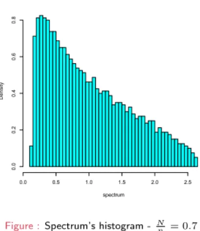
Consider the spectrum of 1nYNY∗Nin the regime where
N, n→ ∞ and N
n →c∈(0,∞) Plot thehistogram of its eigenvalues.
Marˇ cenko-Pastur’s theorem (1967)
”The histogram of aLarge Covariance Matrixconverges to Marˇcenko-Pastur distributionwith given parameter (here0.7)”
13
Histogram for Wishart matrices
: Marˇ cenko-Pastur’s theorem
Matrix model: Wishart matrix
Consider the spectrum of 1nYNY∗Nin the regime where
N, n→ ∞ and N
n →c∈(0,∞) Plot thehistogram of its eigenvalues.
Wishart Matrix, N= 4 ,n= 10
spectrum
Density
0.5 1.0 1.5 2.0 2.5 3.0
0.00.20.40.60.81.01.2
Figure :Spectrum’s histogram -Nn = 0.7
Marˇ cenko-Pastur’s theorem (1967)
”The histogram of aLarge Covariance Matrixconverges to Marˇcenko-Pastur distributionwith given parameter (here0.7)”
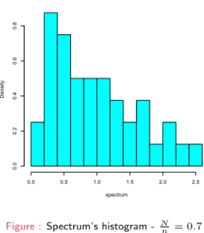
Histogram for Wishart matrices
: Marˇ cenko-Pastur’s theorem
Matrix model: Wishart matrix
Consider the spectrum of 1nYNY∗Nin the regime where
N, n→ ∞ and N
n →c∈(0,∞) Plot thehistogram of its eigenvalues.
Wishart Matrix, N= 40 ,n= 100
spectrum
Density
0.0 0.5 1.0 1.5 2.0 2.5
0.00.20.40.60.8
Figure :Spectrum’s histogram -Nn = 0.7
Marˇ cenko-Pastur’s theorem (1967)
”The histogram of aLarge Covariance Matrixconverges to Marˇcenko-Pastur distributionwith given parameter (here0.7)”
13
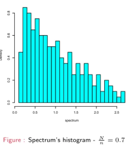
Histogram for Wishart matrices
: Marˇ cenko-Pastur’s theorem
Matrix model: Wishart matrix
Consider the spectrum of 1nYNY∗Nin the regime where
N, n→ ∞ and N
n →c∈(0,∞) Plot thehistogram of its eigenvalues.
Wishart Matrix, N= 200 ,n= 500
spectrum
Density
0.0 0.5 1.0 1.5 2.0 2.5
0.00.20.40.60.8
Figure :Spectrum’s histogram -Nn = 0.7
Marˇ cenko-Pastur’s theorem (1967)
”The histogram of aLarge Covariance Matrixconverges to Marˇcenko-Pastur distributionwith given parameter (here0.7)”
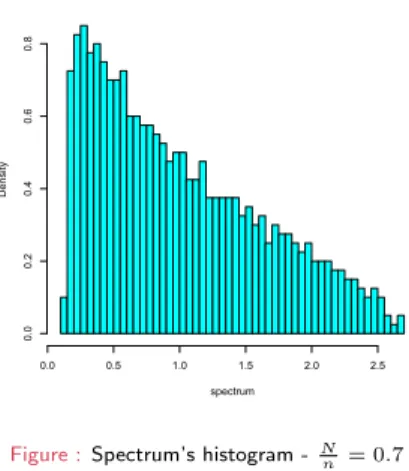
Histogram for Wishart matrices
: Marˇ cenko-Pastur’s theorem
Matrix model: Wishart matrix
Consider the spectrum of 1nYNY∗Nin the regime where
N, n→ ∞ and N
n →c∈(0,∞) Plot thehistogram of its eigenvalues.
Wishart Matrix, N= 800 ,n= 2000
spectrum
Density
0.0 0.5 1.0 1.5 2.0 2.5
0.00.20.40.60.8
Figure :Spectrum’s histogram -Nn = 0.7
Marˇ cenko-Pastur’s theorem (1967)
”The histogram of aLarge Covariance Matrixconverges to Marˇcenko-Pastur distributionwith given parameter (here0.7)”
13
Histogram for Wishart matrices
: Marˇ cenko-Pastur’s theorem
Matrix model: Wishart matrix
Consider the spectrum of 1nYNY∗Nin the regime where
N, n→ ∞ and N
n →c∈(0,∞) Plot thehistogram of its eigenvalues.
Wishart Matrix, N= 1600 ,n= 4000
spectrum
Density
0.0 0.5 1.0 1.5 2.0 2.5
0.00.20.40.60.8
Figure :Spectrum’s histogram -Nn = 0.7
Marˇ cenko-Pastur’s theorem (1967)
”The histogram of aLarge Covariance Matrixconverges to Marˇcenko-Pastur distributionwith given parameter (here0.7)”
Histogram for Wishart matrices: Marˇ cenko-Pastur’s theorem
Matrix model: Wishart matrix
Consider the spectrum of 1nYNY∗Nin the regime where
N, n→ ∞ and N
n →c∈(0,∞) Plot thehistogram of its eigenvalues.
Wishart Matrix, N= 1600 ,n= 4000
spectrum
Density
0.0 0.5 1.0 1.5 2.0 2.5
0.00.20.40.60.8
Figure :Marˇcenko-Pastur’s distribution(in red)
Marˇ cenko-Pastur’s theorem (1967)
”The histogram of aLarge Covariance Matrixconverges to Marˇcenko-Pastur distributionwith given parameter (here0.7)”
13
Elements of proof
1. Convergence of the Stieltjes transform.
Since
LN= 1 N
N
X
i=1
δλi−−−−−−→
N,n→∞ PMPˇ ⇐⇒ gn(z)−−−−−−→
N,n→∞ ST PMPˇ
we prove the convergence ofgn.
2. After algebraic manipulations and probabilistic arguments, we prove that
gn(z)≈ 1
σ2(1−cn)−z−zσ2cngn(z)
3. Necessarily,
gn−−−−−−→
N,n→∞ gMPˇ
which satisfiesthe fixed point equation:
gMPˇ (z) = 1
σ2(1−c)−z−zσ2cgMPˇ (z)
4. Solving explicitely the previous equation, we identify
PMPˇ = (Stieltjes Transform)−1(gMPˇ ).
Elements of proof
1. Convergence of the Stieltjes transform. Since
LN= 1 N
N
X
i=1
δλi−−−−−−→
N,n→∞ PMPˇ ⇐⇒ gn(z)−−−−−−→
N,n→∞ ST PMPˇ
we prove the convergence ofgn.
2. After algebraic manipulations and probabilistic arguments, we prove that
gn(z)≈ 1
σ2(1−cn)−z−zσ2cngn(z)
3. Necessarily,
gn−−−−−−→
N,n→∞ gMPˇ
which satisfiesthe fixed point equation:
gMPˇ (z) = 1
σ2(1−c)−z−zσ2cgMPˇ (z)
4. Solving explicitely the previous equation, we identify
PMPˇ = (Stieltjes Transform)−1(gMPˇ ).
14
Elements of proof
1. Convergence of the Stieltjes transform. Since
LN= 1 N
N
X
i=1
δλi−−−−−−→
N,n→∞ PMPˇ ⇐⇒ gn(z)−−−−−−→
N,n→∞ ST PMPˇ
we prove the convergence ofgn.
2. After algebraic manipulations and probabilistic arguments, we prove that
gn(z)≈ 1
σ2(1−cn)−z−zσ2cngn(z)
3. Necessarily,
gn−−−−−−→
N,n→∞ gMPˇ
which satisfiesthe fixed point equation:
gMPˇ (z) = 1
σ2(1−c)−z−zσ2cgMPˇ (z)
4. Solving explicitely the previous equation, we identify
PMPˇ = (Stieltjes Transform)−1(gMPˇ ).
14
Elements of proof
1. Convergence of the Stieltjes transform. Since
LN= 1 N
N
X
i=1
δλi−−−−−−→
N,n→∞ PMPˇ ⇐⇒ gn(z)−−−−−−→
N,n→∞ ST PMPˇ
we prove the convergence ofgn.
2. After algebraic manipulations and probabilistic arguments, we prove that
gn(z)≈ 1
σ2(1−cn)−z−zσ2cngn(z)
3. Necessarily,
gn−−−−−−→
N,n→∞ gMPˇ
which satisfiesthe fixed point equation:
gMPˇ (z) = 1
σ2(1−c)−z−zσ2cgMPˇ (z)
4. Solving explicitely the previous equation, we identify
PMPˇ = (Stieltjes Transform)−1(gMPˇ ).
Introduction
Large covariance matrices
Wishart matrices and Marˇcenko-Pastur’s theorem The general covariance model
Spiked models
Statistical Test for Single-Source Detection Direction of Arrival Estimation
Conclusion
15
Theorem
Recall the notations
Yn=R1/2N XN and gn(z) = 1 NTrace
1
nYNY∗N−zIN
−1
We are interested in the limiting behaviour of
LN= 1 N
N
X
i=1
δλi with λi=λi
1 nYNY∗N
Canonical equation
I UnknowntN is a Stieltjes transform, solution of
tN(z) = 1
NTrace [(1−cn)RN−zIN−zcntN(z)RN]−1
I Consider associated probabilityPNdefined by
PN = (Stieltjes transform)−1(tN) i.e. tN(z) =
Z PN(d λ) λ−z
Convergence
I ThentN andPNare thedeterminitic equivalentsofgnandLN: gN(z)−tN(z) −−−−−−→a.s.
N,n→∞ 0 and 1 N
N
X
i=1
f(λi)− Z
f(λ)PN(d λ) −−−−−−→a.s.
N,n→∞ 0,
16
Theorem
Recall the notations
Yn=R1/2N XN and gn(z) = 1 NTrace
1
nYNY∗N−zIN
−1
We are interested in the limiting behaviour of
LN= 1 N
N
X
i=1
δλi with λi=λi
1 nYNY∗N
Canonical equation
I UnknowntN is a Stieltjes transform, solution of
tN(z) = 1
NTrace [(1−cn)RN−zIN−zcntN(z)RN]−1
I Consider associated probabilityPNdefined by
PN = (Stieltjes transform)−1(tN) i.e. tN(z) =
Z PN(d λ) λ−z
Convergence
I ThentN andPNare thedeterminitic equivalentsofgnandLN:
gN(z)−tN(z) −−−−−−→a.s.
N,n→∞ 0 and 1 N
N
X
i=1
f(λi)− Z
f(λ)PN(d λ) −−−−−−→a.s.
N,n→∞ 0,
Theorem
Recall the notations
Yn=R1/2N XN and gn(z) = 1 NTrace
1
nYNY∗N−zIN
−1
We are interested in the limiting behaviour of
LN= 1 N
N
X
i=1
δλi with λi=λi
1 nYNY∗N
Canonical equation
I UnknowntN is a Stieltjes transform, solution of
tN(z) = 1
NTrace [(1−cn)RN−zIN−zcntN(z)RN]−1
I Consider associated probabilityPNdefined by
PN = (Stieltjes transform)−1(tN) i.e. tN(z) =
Z PN(d λ) λ−z
Convergence
I ThentN andPNare thedeterminitic equivalentsofgnandLN: gN(z)−tN(z) −−−−−−→a.s.
N,n→∞ 0
and 1 N
N
X
i=1
f(λi)− Z
f(λ)PN(d λ) −−−−−−→a.s.
N,n→∞ 0,
16
Theorem
Recall the notations
Yn=R1/2N XN and gn(z) = 1 NTrace
1
nYNY∗N−zIN
−1
We are interested in the limiting behaviour of
LN= 1 N
N
X
i=1
δλi with λi=λi
1 nYNY∗N
Canonical equation
I UnknowntN is a Stieltjes transform, solution of
tN(z) = 1
NTrace [(1−cn)RN−zIN−zcntN(z)RN]−1
I Consider associated probabilityPNdefined by
PN = (Stieltjes transform)−1(tN) i.e. tN(z) =
Z PN(d λ) λ−z
Convergence
I ThentN andPNare thedeterminitic equivalentsofgnandLN: gN(z)−tN(z) −−−−−−→a.s.
N,n→∞ 0 and 1 N
N
X
i=1
f(λi)− Z
f(λ)PN(d λ) −−−−−−→a.s.
N,n→∞ 0,
Remark
Assume moreover that 1 N
N
X
i=1
δλi(RN)−−−−−−→
N,n→∞ PR
Then instead of having a series ofcanonical equationsdepending onN:
tN(z) = 1
NTrace [(1−cn)RN−zIN−zcntN(z)RN]−1
we can obtain a ”limiting equation”
t(z) =
Z PR(d λ)
(1−c)λ−z−zct(z)λ where t(z) =
Z P∞(d λ) λ−z
and genuine limits
gN(z) −−−−−−→a.s.
N,n→∞ t(z), 1
N
N
X
i=1
f(λi) −−−−−−→a.s.
N,n→∞
Z
f(λ)P∞(d λ),
where theλi’s are the eigenvalues of n1YNYN∗
17
Remark
Assume moreover that 1 N
N
X
i=1
δλi(RN)−−−−−−→
N,n→∞ PR
Then instead of having a series ofcanonical equationsdepending onN:
tN(z) = 1
NTrace [(1−cn)RN−zIN−zcntN(z)RN]−1
we can obtain a ”limiting equation”
t(z) =
Z PR(d λ)
(1−c)λ−z−zct(z)λ where t(z) =
Z P∞(d λ) λ−z
and genuine limits
gN(z) −−−−−−→a.s.
N,n→∞ t(z), 1
N
N
X
i=1
f(λi) −−−−−−→a.s.
N,n→∞
Z
f(λ)P∞(d λ),
where theλi’s are the eigenvalues of n1YNYN∗
17
Remark
Assume moreover that 1 N
N
X
i=1
δλi(RN)−−−−−−→
N,n→∞ PR
Then instead of having a series ofcanonical equationsdepending onN:
tN(z) = 1
NTrace [(1−cn)RN−zIN−zcntN(z)RN]−1
we can obtain a ”limiting equation”
t(z) =
Z PR(d λ)
(1−c)λ−z−zct(z)λ where t(z) =
Z P∞(d λ) λ−z
and genuine limits
gN(z) −−−−−−→a.s.
N,n→∞ t(z),
1 N
N
X
i=1
f(λi) −−−−−−→a.s.
N,n→∞
Z
f(λ)P∞(d λ),
where theλi’s are the eigenvalues of n1YNYN∗
Remark
Assume moreover that 1 N
N
X
i=1
δλi(RN)−−−−−−→
N,n→∞ PR
Then instead of having a series ofcanonical equationsdepending onN:
tN(z) = 1
NTrace [(1−cn)RN−zIN−zcntN(z)RN]−1
we can obtain a ”limiting equation”
t(z) =
Z PR(d λ)
(1−c)λ−z−zct(z)λ where t(z) =
Z P∞(d λ) λ−z
and genuine limits
gN(z) −−−−−−→a.s.
N,n→∞ t(z), 1
N
N
X
i=1
f(λi) −−−−−−→a.s.
N,n→∞
Z
f(λ)P∞(d λ),
where theλi’s are the eigenvalues of n1YNYN∗
17
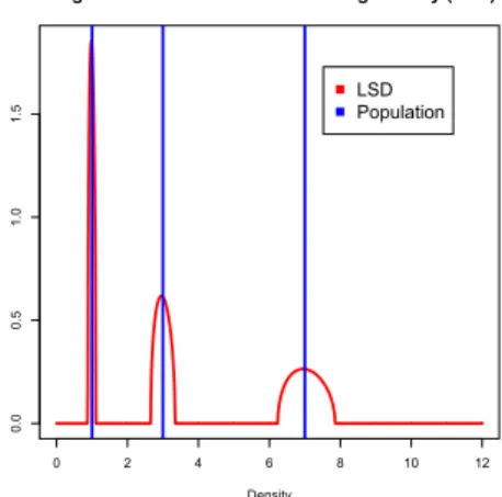
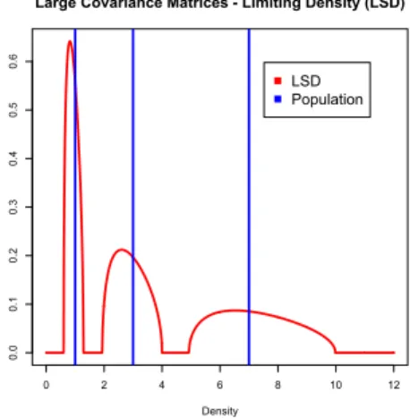
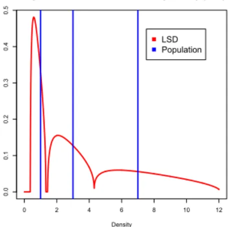
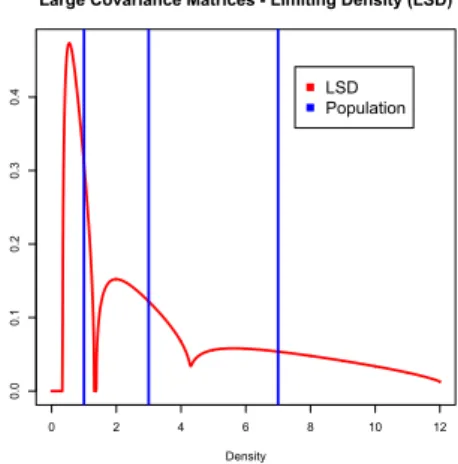
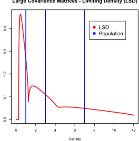
Simulations
I Consider the distribution PR=1
3δ1+1 3δ3+1
3δ7
corresponding to a covariance matrix RN= diag(1,3,7)
each with multiplicity≈N3.
I We plot hereafter the limiting spectral distribution
P∞ for different values ofc.
t(z) =1 3
( 1
(1−c)λ1−z−zct(z)λ1
+ 1
(1−c)λ2−z−zct(z)λ2
+ 1
(1−c)λ3−z−zct(z)λ3 )